Two
Classical Closed-population Capture–Recapture Models
2.1 Introduction
This chapter reviews the classical models for closed populations (i.e., for situations where the individuals in a population remain the same while it is being studied) and the history of their development. The data structure and necessary notation are introduced in section 2.2 via a small data set on the captures of deer mice. Section 2.3 reviews classical two-occasion and multiple-occasion models, i.e., models for situations where two or more than two separate samples of animals are taken. Section 2.4 summarizes the limitations of these classical models and provides motivations for the more general models that are considered in chapter 4.
As noted in chapter 1, the idea of the two-occasion capture–recapture method can be traced to Pierre Laplace, who used it to estimate the human population size of France in 1802 (Cochran 1978), and even earlier to John Graunt who used the idea to estimate the effect of plague and the size of the population of England in the 1600s (Hald 1990). Le Cren (1965) noted that other early applications of this method to ecology included Petersen’s and Dahl’s work on sampling fish populations in 1896 and 1917, respectively, because they recognized that the proportion of previously marked fish captured by fishermen constituted a basis for estimating the population size of the fish. Lincoln was the first to apply the method to wildlife in 1930 when he used returned leg bands from hunters to estimate duck numbers.
Important contributors to the theory of classical closed capture–recapture methods include Schnabel, Darroch, Bailey, Moran, Chapman, and Zippin, among others. The work by Schnabel (1938) and Darroch (1958, 1959) provided the mathematical framework for the models. Detailed historical developments and applications are provided in Cormack (1968), Otis et al. (1978), White et al. (1982), Pollock (1991), Seber (1982, 1986, 1992, 2001), Schwarz and Seber (1999), and Williams et al. (2002).

Figure 2.1. Endangered Néné goose (Nesochen sandvicensis) wearing double leg bands. Island of Maui, Hawaii, 1998. (Photo by Steven C. Amstrup)
2.2 Structure of Capture–Recapture Experiments and Data
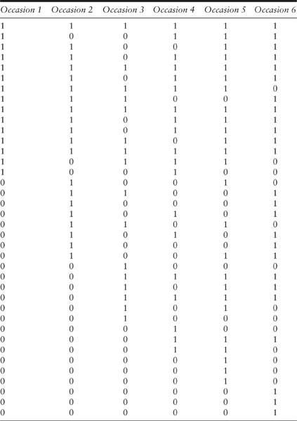
The raw data from closed capture–recapture experiments are the capture records of all the individuals observed in a study. These are arranged in a capture history matrix, as illustrated in table 2.1 with deer mice (Peromyscus sp.) data collected by V. Reid. These data are displayed in the format appropriate for CAPTURE, a widely used computer program for the analysis of closed models (Otis et al. 1978; White et al. 1982; Rexstad and Burnham 1991; section 4.4 of this book). The data arose from a live-trapping experiment that was conducted for six consecutive nights (columns) with a total of 38 mice (rows) captured over these six capture occasions. The time period for the experiment was relatively short and it was reasonable to assume that the population was closed.
In table 2.1, the capture history of each captured individual is expressed as a series of 0’s (noncaptures) and 1’s (captures). Thus, in the example the capture history matrix consists of 38 rows and 6 columns, with the rows representing the capture histories of each captured individual and the columns representing the captures on each occasion. The first mouse, with capture record 111111, was captured on all six nights. The second mouse, with capture record 100111, was captured on nights 1, 4, 5, and 6, but not on nights 2 and 3. Similar interpretations apply to other capture histories.
TABLE 2.1
Individual capture history of 38 deer mice with six capture occasions
In larger studies with numerous capture occasions and many captured individuals, the capture-history matrix becomes very large, and with the classical models it is more convenient to represent the raw data by a tally of the frequencies of each capture history, which retains most of the information in the original capture-history matrix.
For many classical estimation procedures, the following summary statistics are sufficient for the statistical analysis:
k = the number of capture occasions;
nj = the number of animals captured on the jth capture occasion, j = 1, . . . , k;
uj = the number of unmarked animals captured on the jth capture occasion, j = 1, …, k;
mj = the number of marked animals captured on the jth capture occasion, j = 1, …, k, where m1 = 0;
Mj = the number of distinct animals captured before the jth capture occasion, j = 1, …, k, where this is the same as the number of marked animals in the population just before the jth capture occasion, and of necessity M1 = 0 and Mk + 1 is defined as the total number of distinct animals captured in the experiment; and
fj = the number of animals captured exactly j times, j = 1, …, k.
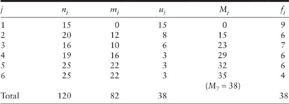
These statistics are given in table 2.2 for the data in table 2.1. The statistic nj denotes the column sum for the jth column (occasion) in the capture history matrix, with (n1, n2, …, n6) = (15, 20, 16, 19, 25, 25). Out of the nj animals, there are uj first captures and mj, recaptures, so that uj + mi = nj, with (u1, u2, …, u6) = (15, 8, 6, 3, 3, 3), and (m1, m2, …, m6) = (0, 12, 10, 16, 22, 22). The statistic Mj can also be interpreted as the cumulative number of first-captures on the first j − 1 occasions, thus Mj = u1 + u2 + … + uj − 1 and (M1, M2, …, M7) = (0, 15, 23, 29, 32, 35, 38). That is, the number of marked individuals in the population progressively increased from M1 = 0 to M7 = 38.
The row sum for each individual denotes the capture frequency of that animal, and (f1, f2, …, fk) represent the frequency counts of all captured animals. As shown in table 2.2, the frequency counts for the mouse data are (f1, f2, …, f6) = (9, 6, 7, 6, 6, 4). That is, 9 animals were captured once, 6 animals captured twice, . . . and 4 animals captured on all 6 occasions. The term f0 is the number of animals never captured, so that f1 + f2 + … + fk = Mk + 1 and f0 + f1 + … + fk = N. Therefore, estimating the population size N is equivalent to estimating the number of missing animals, f0.
TABLE 2.2
Summary statistics for the deer mouse data
2.3 Early Models and Estimators
Some assumptions are common to all closed-population models:
1. The population remains constant over the study period (e.g., there is no immigration or emigration), although known removals (e.g., deaths on capture) are allowed (the closure assumption).
2. Animals do not lose their marks or tags.
3. All marks or tags are correctly recorded.
4. Animals act independently.
Two-occasion Models (Petersen-Lincoln Estimator)
The two-occasion case is the origin of capture–recapture methodology. The intuitive idea is the following: Assume that on the first capture occasion, a sample of n1 animals is captured, marked, and released. Therefore, the marked proportion of the population is
![]()
On the second capture occasion, n2 animals are caught, m2 of which are marked. The proportion of the marked animals in the second sample is m2/n2. Assuming that the marked proportion in the sample is equal to the marked proportion in the population suggests that
![]()
which yields the estimate of the population size
![]()
This is the well-known Petersen-Lincoln estimator, which is also known as the Lincoln-Petersen estimator.
To illustrate this estimator, consider the first two occasions in table 2.1. From table 2.2, n1 = 15, n2 = 20, and m2 = 12, with a total of 23 distinct mice being captured on the first two occasions. The Petersen-Lincoln estimator is then

It appears that this estimate based on capture data from only the first two occasions is not sensible, since a total of 38 distinct mice were actually seen at the end of the experiment.
Various sampling models have been proposed to justify the Petersen-Lincoln estimator and obtain estimates of the associated standard error. A commonly used model assumes a multinomial distribution (section 1.3) under the assumption that on each occasion all animals have the same capture probability (equal catchability). With the multinomial model, the number of captures on each occasion is a random variable. There are three observable capture histories (10, 01, and 11) and three parameters (N, p1, p2), where p1 and p2 denote the capture probabilities for the first and second capture occasions, and the Petersen-Lincoln estimator turns out to be an approximate maximum likelihood estimator (MLE) of N (Seber 1982, p. 131).
Another approach uses the hypergeometric model, and treats the sample sizes n1 and n2 as fixed. This model contains only one parameter N and one random variable m2. Also, under the assumption of equal catchability, the MLE of N is the integer part of the Petersen-Lincoln estimator. If n1 + n2 ≥ N, then an unbiased estimator proposed by Chapman (1951) is
![]()
An intuitive explanation for why this estimator can reduce bias is that the bias of the Petersen-Lincoln estimator is mainly due to small values of m2, especially m2 = 0. This means no animals are captured twice, and the estimate of equation 2.1 is infinite. Hence, one extra animal is added into the frequency of animals caught on both occasions so that m2 is at least one, and n1, n2 and the population size are consequently all increased by one. Chapman’s estimator follows from the fact that (n1 + 1) × (n2 + 1)/(m2 + 1) is a valid estimator for N + 1. When n1 + n2 < N, the bias of Chapman’s estimator is approximately equal to − Nexp[−(n1 + 1) × (n2 + 1)/N] (Seber 1982, p. 60). There are other bias-corrected estimators. For example, Bailey (1951, 1952) adopted a binomial model and obtained a different bias-corrected estimator.
The difference between the Petersen-Lincoln and Chapman’s estimator is small when the number of recaptures is not small relative to n1 and n2. For example, Chapman’s estimate based on the first two capture occasions of table 2.1 is

compared to the Petersen-Lincoln estimate of 25.
Both estimators have approximately the same variance formula, given by

(Seber 1982, p. 60). Hence, the variances are approximately 16 × 21 × 3 × 8/(13 × 13 × 14) = 3.41 and the approximate standard error is ![]() . A traditional 95% confidence interval based on Chapman’s estimator and the large-sample normal approximation can therefore be calculated as 24.85 ± 1.96 × 1.85 = (21, 29). This interval clearly cannot cover the true population size because 38 animals were actually captured in the experiment. Suppose that only the data for the first two occasions are available, a drawback for the traditional confidence interval is that the lower limit of this interval is less than the observed number of animals, which is 23 in this case. A modification is to replace the lower bound by the number of captured. That is, the resulting interval is modified to (23, 29) based on the first two occasions. More discussion on interval estimation is presented in chapter 4.
. A traditional 95% confidence interval based on Chapman’s estimator and the large-sample normal approximation can therefore be calculated as 24.85 ± 1.96 × 1.85 = (21, 29). This interval clearly cannot cover the true population size because 38 animals were actually captured in the experiment. Suppose that only the data for the first two occasions are available, a drawback for the traditional confidence interval is that the lower limit of this interval is less than the observed number of animals, which is 23 in this case. A modification is to replace the lower bound by the number of captured. That is, the resulting interval is modified to (23, 29) based on the first two occasions. More discussion on interval estimation is presented in chapter 4.
Multiple-recapture Models (The Schnabel Census)
As noted above, two capture occasions may not result in reliable estimates. Two-occasion models were extended to multiple occasions by Schnabel (1938) and Darroch (1958). Their approaches formed the basis of the classical models. Like the Petersen-Lincoln model, these early models assume that on each sampling occasion all animals have the same probability of capture, although this probability can be allowed to vary among sampling occasions. The models have been extensively discussed in the literature because the capture probabilities may vary with environmental conditions or the sampling effort. Because the sample data taken on the k occasions are statistically independent under the assumption of equal catchability, this model is also referred to as an “independent” model in the literature.
A special case of the equal catchability model is where the capture probability p is constant over the capture occasions. This is usually referred to as model M0, the subscript 0 referring to no variation. Then, for example, for the data in table 2.1, the probability of an animal having the capture history 111111 is p6; the probability of an animal having the capture history 100111 is p4(1 − p)2, and the probability an animal is not captured is (1 − p)6. As discussed in section 1.3, by considering all possible capture histories and the corresponding counts, the likelihood based on a multinomial model becomes in this case
![]()
where ah denotes the frequency for observable capture history h and n = n1 + n2+ … + nk denotes the total number of captures, which is 120 for the example.
In model M0, there are only the two parameters, N and p, and the statistics that are necessary to estimate them are Mk + 1 and n . The MLE of N and p can be obtained using numerical methods that maximize equation 2.4. A large-sample variance (Darroch 1958) is obtained by substituting the estimates into the formula

For the data in table 2.1, the MLE are ![]() = 0.526 and
= 0.526 and ![]() = 38 (standard error = 0.69). After model M0 is applied it is concluded that nearly all animals were caught, with a narrow 95% confidence interval of (38, 39.4) for the true population size.
= 38 (standard error = 0.69). After model M0 is applied it is concluded that nearly all animals were caught, with a narrow 95% confidence interval of (38, 39.4) for the true population size.
This simple model, however, does not fit the data properly. Although more rigorous statistical tests (to be discussed below) are not possible for this data set due to the sparse counts, the fitted (expected) values shown in table 2.3 do help to check the model. Because the model assumes that the capture probabilities are the same for all k occasions, the fitted values for the numbers of captures on the six occasions are equal, i.e., E(n1) = E(n2) = · = E(n6) = 20. The other fitted values follow from the formulas E(uj) = N(1 − p)j − 1 p and E(mj) = N[1 − (1 — p)j − 1]p. With model M0, it is expected that the number of new animals captured will decrease rapidly from 20 to 0.5, but the data did not show such a trend. The counts (u1, u2, …, u6, f0) follow a multinomial distribution, and thus the usual chi-squared goodness-of-fit test can be applied. Pooling u4, u5, u6, and f0, we have four observed cells (u1, u2, u3, u4 + u5 + u6 + f0) = (15, 8, 6, 9). Here f0 = 0 because the population size estimate is 38. Note that E(u4 + u5 + u6 + f0) = ![]() − E(u1 + u2 + u3), and it follows from table 2.3 that the corresponding expected values are (20.0, 9.47, 4.49, 4.04) with
− E(u1 + u2 + u3), and it follows from table 2.3 that the corresponding expected values are (20.0, 9.47, 4.49, 4.04) with ![]() = 38. Then the chi-squared value is 8.08 with 1 degree of freedom. The p value is 0.004, which reveals that the model is not adequate. Here the degree of freedom for the test is equal to the number of cells −1 −r, where r denotes the number of parameters, which is r = 2 under model M0.
= 38. Then the chi-squared value is 8.08 with 1 degree of freedom. The p value is 0.004, which reveals that the model is not adequate. Here the degree of freedom for the test is equal to the number of cells −1 −r, where r denotes the number of parameters, which is r = 2 under model M0.
TABLE 2.3
Fitted (expected) values for deer mouse data for two models

If we modify the classical model to allow capture probabilities to vary with time, we refer to it as model Mt, where the subscript t refers to variation of the capture probabilities over time. Denote the capture probability for all individual animals on the jth occasion by pj. The likelihood for the special case of k = 3 was presented in section 1.3. The extension to any number of occasions is similar. Unlike model M0, where only one parameter is used to model the capture probability, if there are k capture occasions, then model Mt uses the k parameters p1, p2, …, pk to describe the capture probabilities. For example in table 2.1, the probability for an animal having capture history 111111 is p1p2p3p4p5p6; the probability for an animal having capture history 100111 is p1(1 − p2) × (1 − p3)p4p5p6 …; and the probability an animal is not captured is (1 — p1)(1 · p2)(1 − P3)(1 − P4)(1 − P5)(1 − p6). The multinomial likelihood representing an extension of equation 2.1 turns out to be

There are k + 1 parameters (N, p1, p2, …, pk) and the statistics needed to estimate these are (n1, n2, …, nk, Mk + 1). The iterative procedure for finding the exact MLE is described by Otis et al. (1978, p. 106) and the variance is then approximately given by

For the data of table 2.1, the capture probabilities are respectively estimated by ![]() 1 = 0.395,
1 = 0.395, ![]() 2 = 0.526,
2 = 0.526, ![]() 3 = 0.421,
3 = 0.421, ![]() 4 = 0.50,
4 = 0.50, ![]() 5 =
5 = ![]() 6 = 0.658 and the MLE of N is 38 with an estimated standard error of 0.62. This classical model Mt also indicates that nearly all of the mice were caught and a traditional 95% confidence interval indicates that at most one mouse was missed. The fitted values of this model are shown in table 2.3. Because there are six parameters to model six capture probabilities, the fitted number of captures on each occasion matches the data, i.e., E(nj) = nj, for j = 1, 2, …, 6. The other fitted values are based on
6 = 0.658 and the MLE of N is 38 with an estimated standard error of 0.62. This classical model Mt also indicates that nearly all of the mice were caught and a traditional 95% confidence interval indicates that at most one mouse was missed. The fitted values of this model are shown in table 2.3. Because there are six parameters to model six capture probabilities, the fitted number of captures on each occasion matches the data, i.e., E(nj) = nj, for j = 1, 2, …, 6. The other fitted values are based on
![]()
and
![]()
Under model Mt, the usual chi-squared goodness-of-fit test for multinomial counts cannot be computed due to sparseness of the data and relatively many parameters. Although the model is an extension of model M0, a new chi-square goodness of fit test proposed by Stanley and Burnham (1999, p. 373) shows that this classical model still cannot provide a good fit to the data (chi-squared = 18.67, with 11 degrees of freedom, p = 0.067). Therefore, neither of the models M0 and Mt appears suitable for the data.
Tests of Equal Catchability
With model Mt, a basic assumption is all animals have the same probability of capture at each sampling occasion. Equal catchability may be an unattainable ideal with naturally occurring wild populations. Under some circumstances, however, the effects of violating this assumption can be assessed, and the resulting biases may not be too severe (Carothers 1973a).
If there are only two capture occasions, the equal catchability assumption is not testable because with two occasions there are three parameters and three observable capture frequencies with the multinomial model. Therefore, no degrees of freedom are left for the test of goodness of fit. For more than two occasions, Seber (1982, p.157) described the usual chi-squared goodness-of-fit test for all observed capture frequencies. Large-scale pooling may be necessary to perform this chi-squared test when counts are sparse. A test proposed by Leslie (1958) and further described by Otis et al. (1978, pp. 118–119) and Krebs (1999, section 2.4) has been widely used. However, this test also requires a large number of data. Stanley and Burnham (1999) recently reviewed the available tests of catchability and proposed a more efficient approach.
Causes and Consequences of Assumption Failures
There are two common causes for the failure of the equal catchability assumption:
1. The capture probability of an animal depends on its previous capture history. For example, animals may become either trap happy or trap shy if trapping methods are kept constant. Marked animals that have a higher probability of being captured (e.g., because they are attracted by the bait) on subsequent occasions would be called trap happy. On the other hand, marked animals may become trap shy because of the unpleasant experience of being captured. The recapture probability on subsequent capture occasions thus becomes lower than that for uncaptured animals.
2. The capture probability is a property of the animal and thus the individual capture probabilities may be heterogeneous across the individuals in a population. Individual capture probabilities may vary with age, sex, body weight, activity, the number of traps near the home range, or other unobservable individual characteristics. For example, studies have shown that for some species the males are consistently more likely to be caught than the females and young animals are more catchable than subadults or adults.
The above two causes are usually mixed and cannot be easily disentangled in a data analysis. Violation of the equal catchability assumption leads to biases for the usual Petersen-Lincoln and Chapman’s estimators. For example, if animals exhibit a trap-happy behavioral response or if individual heterogeneity exists and is consistent over sampling occasions, then the animals captured in the first sample are more easily caught in the second sample. Thus, the recapture rate (m2/n2) in the second sample tends to be larger than the true proportion of marked animals in the population n1/N. Then it is expected that m2/n2 > n1/N, which yields N > n1n2/m2 = ![]() p. As a result, the Petersen-Lincoln estimator tends to underestimate the true size. Conversely, it tends to overestimate with the trap-shy animals. Similar arguments and conclusions are also valid for more than two capture occasions.
p. As a result, the Petersen-Lincoln estimator tends to underestimate the true size. Conversely, it tends to overestimate with the trap-shy animals. Similar arguments and conclusions are also valid for more than two capture occasions.
Classical Resolution of Problems Resulting from Assumption Failures
Behavioral response is usually induced by the use of identical trapping methods over the capture occasions. To reduce this effect the use of different trapping methods has been proposed, for example, trapping and then resighting in wildlife studies, or netting and then angling in fishery science. However, this is sometimes infeasible if a number of trapping occasions are used or if available trapping options are limited by costs or logistical constraints.
Some common sources of heterogeneity are observable and can be recorded, e.g., the age, sex, or other characteristics of the individual animals. Such sources can then be eliminated by stratification. That is, analyses are performed within subsets of the data that are homogeneous with regard to the characteristics of animals. However, when there are many stratifying factors, the data in each stratum become sparse. Also, when heterogeneity is due to unobservable or inherent attributes, then residual heterogeneity may still exist even within strata.
2.4 Limitations of Early Models and the Motivation for More General Models
The classical model Mt assumes that all animals have the same probabilities of capture on any particular occasion, though the probability may vary from one occasion to another. The usual estimators under classic models often are either negatively biased (in the trap-happy cases or when heterogeneity exists) or positively biased (in the trap-shy cases). Although these estimators may have good precision (a small variance) and produce narrow confidence intervals, these intervals may be too optimistic and do not reveal their bias. Therefore, models assuming equal catchability may often result in misleading interpretation of the data. In some cases biases resulting from assumption violations may be small and have little impact on study conclusions. It is critical for the investigator, therefore, to be familiar enough with the data and the study situation to interpret data and results of analyses in light of necessary caveats.
Although different sampling methods or stratified analyses have been suggested to minimize trap-response effects or heterogeneity, these suggestions have practical limitations. Therefore, more complex models that allow for unequal catchabilities are needed. These are discussed in chapter 4.

Figure 2.2. Fin-clipping Dolly Varden (Salvelinus malma malma) to test retention of Floy Anchor Tag (center of photo), Buskin River, Kodiak Island, Alaska, 1992. (Photo by Mary Whalen)
2.5 Chapter Summary
• The early history of methods for the estimation of the size of a closed population from capture–recapture data is reviewed, beginning with the work of Graunt about 400 years ago and Laplace about 200 years ago. The form of capture–recapture data is described, with the statistics that are often used to summarize the data for an analysis.
• The common assumptions of capture–recapture models are listed (a constant population size, no loss of marks, correct recording of marks, and animals behave independently).
• The classical Petersen-Lincoln estimator of population size is described and its variance and bias given.
• The Schnabel census with more than two sampling occasions is described with the models M0 (constant capture probabilities) and Mt (capture probabilities vary with time) used for estimation. Variance equations are provided for both models. Their use is illustrated on a data set involving the captures of deer mice with six sampling occasions.
• Tests are described for the assumption that all animals have the same probability of being captured.
• The causes and consequences of failures of assumptions are discussed, together with ways to avoid the effects of failures. The need for more complicated models as covered in chapter 4 is highlighted.