One
Introduction to the Handbook
1.1 Introduction
In September of 1802, Pierre Simon Laplace (1749–1827) used a capture–recapture type of approach to estimate the size of the human population of France (Cochran 1978; Stigler 1986). At that time, live births were recorded for all of France on an annual basis. In the year prior to September 1802, Laplace estimated the number of such births to be approximately X = 1,000,000. These newly born individuals constituted a marked population. Laplace then obtained census and live birth data from several communities “with zealous and intelligent mayors” across all of France. Recognizing some variation in annual birth rates, Laplace summed the number of births reported in these sample communities for the three years leading up to the time of his estimate, and divided by three to determine that there were x = 71,866 births per year (marked individuals) in those communities. The ratio of these marked individuals to the total number of individuals in the sampled communities, y = 2,037,615 was then the estimate

of the proportion of the total population of France that was newly born. On this basis, the one million marked individuals in the whole of France is related to the total population N as
![]()
so that
![]()

Figure 1.1. Jeff Mason fires a shoulder-held cannon net used to capture Bristle-thighed Curlews (Numenius tahitiensis) on the Seward Peninsula, spring 1989. (Photo by Robert Gill)
This estimation procedure is equivalent to the Lincoln-Peterson capture–recapture estimator described in chapter 2.
Although Laplace is commonly thought of as the first to use the capture–recapture idea, he was preceded by almost 200 years by John Graunt in his attempts to use similar methods to estimate the effect of plague and the size of populations in England in the early 1600s (Hald 1990). The theories and applications of capture–recapture have moved far beyond the concepts of John Graunt and Pierre Laplace in the ensuing centuries. Current methods do, however, share the basic concept, of ratios between known and unknown values, that guided those pioneers.
Our purpose in this book is to provide a guide for analyzing capture–recapture data that can lead the naive reader through basic methods, similar to those used by the earliest of workers, to an understanding of modern state of the art methods. This handbook is intended primarily for biologists who are using or could use capture–recapture to study wildlife populations. To the extent practicable, therefore, we have kept mathematical details to a minimum. We also have, beginning with this first chapter, attempted to explain some of the mathematical details that are necessary for a complete conceptual understanding of the methodologies described. Also, authors of each chapter have been encouraged to provide all the references that are necessary to enable readers to obtain more details about the derivations of the methods that are discussed. Therefore, this book also will be a useful introduction to this subject for statistics students, and a comprehensive summary of methodologies for practicing biometricians and statisticians.
The book is composed of three sections. Section 1 is this chapter, which is intended to set the scene for the remainder of the book, to cover some general methods that are used many times in later chapters, and to establish a common notation for all chapters. Section 2 consists of seven chapters covering the theory for the main areas of mark–recapture methods. These chapters contain some examples to illustrate the analytical techniques presented. Section 3 consists of two chapters in which we explicitly describe some examples of data sets analyzed by the methods described in chapters 2 to 8. When useful throughout the book, we discuss computing considerations, and comment on the utility of the different methods.
1.2 Overview of Chapters 2 to 8
Chapters 2 to 8 cover the main methods available for the analysis of capture–recapture models. For those who are unfamiliar with these methods the following overviews of the chapters should be useful for clarifying the relationships between them. Figure 1.2 contains a flowchart of the capture–recapture methods described in this section of the book. This flowchart may help to clarify the relationship between analyses, and will indicate the chapter (or section) containing methods appropriate for a particular data set.
Closed-population Models
A closed population is one in which the total number of individuals is not changing through births, deaths, immigration, or emigration. The first applications of capture–recapture methods were with populations that were assumed to be closed for the period of estimation. It is therefore appropriate that the first chapter in section 2 of this book should describe closed-population models. In practice, most real populations are not closed. Sometimes, however, the changes over the time period of interest are small enough that the assumption of closure is a reasonable approximation, and the effects of violating that assumption are minimal. For this reason, the analysis of capture–recapture data from closed populations continues to be a topic of interest to biologists and managers.
In chapter 2, Anne Chao and Richard Huggins begin by discussing some of the early applications of the capture–recapture method with one sample to mark some of the individuals in a population, and a second sample to see how many marked animals are recaptured. The data obtained from the two samples can be used to estimate the population size.
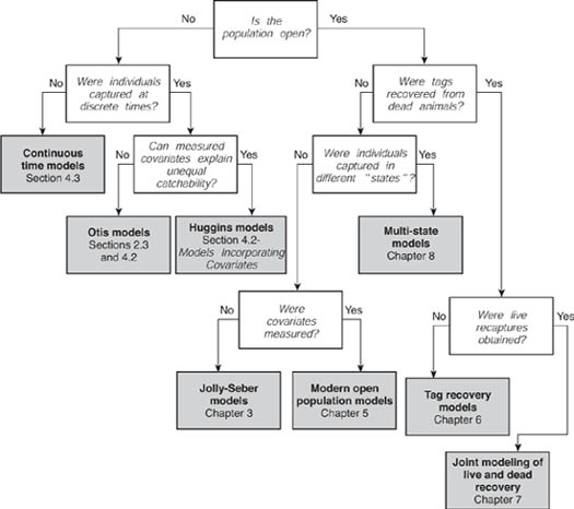
Figure 1.2. Flowchart of the methods described in this book. Starting with Is the population open?, unshaded boxes present Yes/No questions about the characteristics of the capture–recapture study and data. The paths induced by answers to these questions terminate at shaded boxes, which give the applicable models and this volume’s chapter or section reference.
A natural extension of the two-sample method, which can be traced back to Schnabel (1938), involves taking three or more samples from a population, with individuals being marked when they are first caught. The analysis of data resulting from such repeated samples, all within a time period during which the population is considered closed, is also considered in chapter 2. The goal still is estimation of the population size, but there are many more models that can be applied in terms of modeling the data. Chao and Huggins therefore conclude chapter 2 by noting the need for more general models.
The discussion is continued by Chao and Huggins in chapter 4. There they consider how the probability of capture can be allowed to vary with time, the capture history of an animal, and different animals, through the Otis et al. (1978) series of models. Other topics that are covered by Chao and Huggins in chapter 4 are the incorporation of covariates that may account for variation in capture probabilities related to different types of individuals (e.g., different ages or different sexes) or different sample times (e.g., the sampling effort or a measure of weather conditions), and a range of new approaches that have been proposed for obtaining population size estimates.
Basic Open-population Models
An open population is one that is (or could be) changing during the course of a study, because of any combination of births, deaths, immigration, or emigration. Because most natural wildlife populations are affected in this way, the interest in using capture–recapture data with open populations goes back to the first half of the 20th century when ecologists such as Jackson (1939) were sampling populations that were open, and developing methods for estimating the changing population sizes, the survival rates, and the number of individuals entering the populations between sample times.
A major achievement was the introduction of maximum likelihood estimation for the analysis of open-population capture–recapture data by Cormack (1964), Jolly (1965), and Seber (1965). This led to the development of what are now called the Cormack-Jolly-Seber (CJS) and the Jolly-Seber (JS) models. The CJS model is based solely on recaptures of marked animals and provides estimates of survival and capture probabilities only. The JS model incorporates ratios of marked to unmarked animals and thereby provides estimates of population sizes as well as survival and capture probabilities. The fundamental difference between the two is that the JS model incorporates the assumption that all animals are randomly sampled from the population and that captures of marked and unmarked animals are equally probable. The CJS model, on the other hand, does not make those assumptions and examines only the recapture histories of animals previously marked.
The CJS and JS models are the main topics of chapter 3 by Kenneth H. Pollock and Russell Alpizar-Jara. For the JS model, equations are provided for estimates of population sizes at sample times, survival rates between sample times, and numbers entering between sample times. In addition, there is a discussion of versions of this model that are restricted in various ways (e.g., assuming constant survival probabilities or constant capture probabilities) or generalized (e.g., allowing parameters to depend on the age of animals). The CJS model, which utilizes only information on the recaptures of marked animals, is then discussed. As noted above, this model has the advantage of not requiring unmarked animals to be randomly sampled from the population, but the disadvantage that this allows only survival and capture probabilities to be estimated. Population sizes, which were the original interest with capture–recapture methods, cannot be directly estimated without the random sampling, which allows extrapolation from the marked to the unmarked animals in the population.
Recent Developments with Open-population Models
Since the derivation of the original CJS and JS models there have been many further developments for modeling open populations, which are covered by James D. Nichols in chapter 5. These developments are primarily due to the increasing availability of powerful computers, which make more flexible, but also much more complicated, modeling procedures possible. Parameter values can be restricted in various ways or allowed to depend on covariates related either to the individuals sampled or to the sample time.
The flexible modeling makes it possible to consider very large numbers of possible models for a set of capture–recapture data, particularly if the animals and sample times have values of covariates associated with them. The larger number of possible models that can be considered with modern computerized approaches elevates the importance of objective model selection procedures that test how well each model fits the data. It always has been necessary to assess whether models were apt, how well they fit the data, and which of the models should be considered for final selection. Our greater ability now to build a variety of models is accompanied by a greater responsibility among researchers and managers to perform the comparisons necessary so that the best and most appropriate models are chosen.
The methodological developments in chapter 5 were motivated primarily by biological questions and the need to make earlier models more biologically relevant. This underlying desire to generalize and extend the CJS model resulted in several new models. These methods, covered in chapter 5, include reverse-time modeling, which allows population growth rates to be estimated; the estimation of population sizes on the assumption that unmarked animals are randomly sampled; models that include both survival and recruitment probabilities; and the robust design in which intense sampling is done during several short windows of time (to meet the assumption of closure) that are separated by longer intervals of time during which processes of birth, death, immigration, and emigration may occur. Population size estimates are derived from capture records during the short time periods of the robust design, and survival is estimated over the longer intervals between periods.
Tag-recovery Models
The tag-recovery models that are discussed by John M. Hoenig, Kenneth H. Pollock, and William Hearn in chapter 6 were originally developed separately from models for capture–recapture data. These models are primarily for analyzing data obtained from bird-banding and fish-tagging studies. In bird-banding studies, groups of birds are banded each year for several years and some of the bands are recovered from dead birds, while in fish-tagging studies, groups of fish are tagged and then some of them are recovered later during fishing operations. The early development of tag-recovery models was started by Seber (1962), and an important milestone was the publication of a handbook by Brownie et al. (1978) in which the methods available at that time were summarized.
The basic idea behind tag-recovery models is that for a band to be recovered during the jth year of a study, the animal concerned must survive for j − 1 years, die in the next year, and its band be recovered. This differs from the situation with capture–recapture data where groups of animals are tagged on a number of occasions and then some of them are recaptured later while they are still alive.
Joint Modeling of Tag-recovery and Live-recapture or Resighting Data
It is noted above that the difference between standard capture–recapture studies and tag-return studies is that the recaptures are of live animals in the first case, while tags are recovered from dead animals in the second case. In practice, however, the samples of animals collected for tagging do sometimes contain previously tagged animals, in which case the study provides both tag-return data and data of the type that comes from standard capture–recapture sampling.
If there are few recaptures of live animals, they will contribute little information and can be ignored. If there are many live recaptures, however, it is unsatisfactory to ignore the information they could contribute to analyses, leading to the need for the consideration of methods that can use all of the data. This is the subject of chapter 7 by Richard J. Barker, who considers studies in which animals can be recorded after their initial tagging (1) by live recaptures during tagging operations, (2) by live resightings at any time between tagging operations, and (3) from tags recovered from animals killed or found dead between tagging occasions. In addition to describing the early approaches to modeling these types of data, which go back to papers by Anderson and Sterling (1974) and Mardekian and McDonald (1981), Barker also considers the use of covariates, model selection, testing for goodness of fit, and the effects of tag loss.
Multistate Models
The original models of Cormack (1964), Jolly (1965), and Seber (1965) for capture–recapture data assumed that the animals in the population being considered were homogeneous in the sense that every one has the same probability of being captured when a sample was taken, and the same probability of surviving between two sample times. Later, the homogeneity assumption was relaxed, with covariates being used to describe different capture and survival probabilities among animals. However, this still does not allow for spatial separation of animals into different groups, with random movement between these groups. For example, consider an animal population in which members move among different geographic locales (e.g., feeding, breeding, or molting areas). Also consider that survival and capture probabilities differ at each locale. Covariates associated with the individual animals or sample times are insufficient to model this situation, and the movement between locations must be modeled directly.
In chapter 8, Carl J. Schwarz considers the analysis of studies of this type, where the population is stratified and animals can move among strata or states while sampling takes place. Analyses for these types of situations were first considered by Chapman and Junge (1956) for two samples from a closed population, extended for three samples from an open population by Arnason (1972, 1973), and to k samples from an open population by Schwarz et al. (1993b) and Brownie et al. (1993). These models can be used to study dispersal, migration, metapopulations, etc. Although the models were developed primarily to account for the physical movement of animals among geographic strata, the models described in chapter 8 also work where states are behavioral (e.g., breeding or nonbreeding animals each of which may be more or less available than the other) or habitat related rather than just geographic. Chapter 8 also shows how live and dead recoveries can be treated as different states, and describes how covariates that change randomly with time can be used to describe individuals in different states.
The first part of chapter 8 deals with the estimation of migration, capture, and survival probabilities for a stratified population, using a generalization of the Cormack-Jolly-Seber model. The last part considers the estimation of population size using two or several samples from a stratified closed population, and using several samples from an open population.
1.3 Maximum Likelihood with Capture–Recapture Methods
Early methods for analyzing capture–recapture and tag-recovery data relied upon ad hoc models for their justification. However, by the late 1960s the use of well-defined probability models with maximum likelihood estimation of the unknown parameters had become the standard approach. The method of maximum likelihood, which is known to produce estimates with good properties under a wide range of conditions, consists of two steps. First, there is the construction of a model that states the probability of observing the data as a function of the unknown parameters that are of interest. This is called the likelihood function. Second, the estimates of the unknown parameters are chosen to be those values that make the likelihood function as large as possible, i.e., the values that maximize the likelihood.
For the data considered in this book, three related types of likelihood functions need to be considered. The first and simplest arises by modeling the probability of observing the data from single independent animals, and then constructing the full likelihood as the product of probabilities for all animals. The second type of likelihood arises when data are grouped, which leads to use of the multinomial distribution to describe the probability of observing all the capture data. The third type of likelihood arises when data are collected from independent groups, which leads to likelihoods that are the product of multinomial distributions.
To illustrate the first type of likelihood, consider a four-sample experiment where n1 animals are marked in the first sample, no more marking is done, and recapture data are obtained during samples 2, 3, and 4. Suppose that the probability of an animal surviving from the time of the jth sample to the time of the next sample is ϕj (j = 1, 2, or 3), and the probability of a live animal being captured in the jth sample is pj. Assume further that a particular animal was captured on the first capture occasion, and resighted on the third and fourth capture occasions. The history of captures and resightings for this animal can be indicated by the pattern of digits 1011, where a 1 in the jth position (counting from the left) indicates capture or resight during the jth occasion, and 0 in the jth position indicates that the animal was not seen during the jth occasion. Under these assumptions, the probability of observing this particular pattern of resightings, conditional on the original capture, is
![]()
which is obtained by multiplying together the probabilities of surviving until the second sample (ϕ1), not being captured in the second sample (1 − p2), surviving from the second to third sample times (p3), getting captured in the third sample (ϕ3), surviving from the third to fourth sample times (ϕ3), and finally getting captured in the fourth sample (p4).
Probabilities of capture and survival for each animal in a series of samples can be used to describe the probabilities of their capture histories as in equation 1.1. The likelihood of observing all of the data is then the product of the probabilities, i.e.,

where Pj is the probability for the jth animal, assuming that the history for each animal is independent of the history for all of the other animals. Maximum likelihood estimation would involve finding the values of the survival and capture probabilities that maximize L. Note that ϕ3 and p4 cannot be estimated individually in this example because it is not possible to tell whether a large number of captured animals in the fourth and last sample is due to a high survival rate from the previous sample time or a high probability of capture. Therefore, only the product ϕ3p4 can estimated. Similarly, the capture probability cannot be estimated for the first occasion. In general, this sort of limitation applies at both ends of capture–recapture histories.
The second type of likelihood is for grouped data. In this case, the multinomial distribution is used to give the probability of the observed data. With this distribution there are m possible types of observation, with the ith type having a probability θi of occurring, where
![]()
If there is a total sample size of n, with ni observations of type i occurring so that n = n1 + n2 + … + nm, then the multinomial distribution gives the probability of the sample outcome (the likelihood) to be
![]()
a probability statement that is justified in many elementary statistics texts.
Typically, when a multinomial likelihood function like this occurs in the following chapters then the θ parameters will themselves be functions of other parameters, which are the ones of real interest. For example, consider a three-sample capture–recapture study on a closed population of size N, with a capture probability of pi for the ith sample. The possible capture–recapture patterns with their probabilities are then

and
![]()
If ni observations are made of the ith capture–recapture pattern, then the likelihood function would be given by equation 1.3, with the θ values being functions of the p values, as shown above. In addition, because the number of uncaptured animals is unknown, this must be set equal to n1 = N − n2 − n3 − … − n8 in equation 1.3. Maximum likelihood estimates of N, p1, p2, and p3 would then be found by maximizing the likelihood with respect to these four parameters.
The third type of likelihood function occurs when the probability of the observed data is given by two or more multinomial probabilities like (1.3) multiplied together. This would be the case, for example, if the three-sample experiment just described was carried out with the results recorded separately for males and females. In that case there would be one multinomial likelihood for the males and another for the females. The likelihood for all the data would then be the product of these two multinomials. The parameters to be estimated would then be the number of males, the number of females, and capture probabilities that might or might not vary for males and females.
Likelihood Example 1
In this and the next example we illustrate some of the calculations involved in the maximum likelihood method. These examples are designed to provide the reader with a better understanding of what is meant by the phrase “estimates can be obtained by maximum likelihood” when it is used in later chapters. They are by no means a full treatment of the maximum likelihood method, but should be sufficient to provide readers with a clearer idea of the methodology behind many of the capture–recapture estimates mentioned later.
Once a likelihood for the observed data is specified, the second step in the maximum likelihood estimation process is to maximize the likelihood to obtain parameter estimates. To illustrate this second step consider again the four-sample capture–recapture experiment described above for the first type of likelihood. Suppose that n1 = 2 animals are captured and marked in the first sample, and that one of these animals is recaptured in samples three and four, while the other animal is only recaptured in sample four. The capture histories for these two animals are then represented by 1011 and 1001.
Following similar logic to that used to derive equation 1.1, the probabilities of the individual capture histories are
![]()
and
![]()
Assuming that the results for the two captured animals were independently obtained, the full likelihood of obtaining both the capture histories is

Typically, the natural logarithm of L is taken at this point because L and ln(L) are maximized by the same parameter values, and the logarithmic function ln(L) is generally easier to maximize on a computer. The log-likelihood for this example is

The process of “maximizing the likelihood” essentially entails repeatedly modifying the values of ϕi and pi until ln(L) cannot be increased any more. To start the process, a set of initial parameters is defined. In this example, suppose that the maximization process is started with ϕi = 0.5 for all i, and pi = 0.5 for all i. Putting these initial values into ln(L) gives

It is then possible to get progressively closer to the final maximum by a judicious choice of the changes to make to the parameters. In particular, using the theory of calculus it is possible to determine the direction to change each of the parameters so that ln(L) will increase. However, the magnitude of the changes that will assure that the new values produce the maximum is not known. Consequently, small changes in the parameters are made until further changes will not increase ln(L).
The technique relies on the calculation of the derivatives of ln(L) with respect to the parameters, to specify which changes in the parameters will increase ln(L). These details are explained in texts on calculus, but are unnecessary here. For illustrating the calculations, all one needs to know is that the derivatives for the example being considered specify that changing the parameter estimates to ϕ1 = 0.55, ϕ2 = 0.55, ϕ3 = 0.55, p2 = 0.45, p3 = 0.50, and p4 = 0.55 will increase ln(L). To check this, these values can be used to calculate ln(L), which gives
Repeating the process of calculating the gradient and changing the parameter estimates will eventually maximize ln(L). For example, the new derivatives calculated at the last parameter values specify that changing the parameter estimates to ϕ1 = 0.59, ϕ2 = 0.59, ϕ3 = 0.59, p2 = 0.41, p3 = 0.50 and p4 = 0.59 will increase ln(L). The ln(L) value with these new parameter estimates is − 6.66.
In this particular example, the likelihood is overparameterized because there are six parameters and only two capture histories. Overparameterization causes a number of problems, and, in particular, means that some parameters must be assigned arbitrary values to fix the other parameters. This overparameterized likelihood was used here, however, only to illustrate calculation of individual ln(L) values. In the next section, more capture histories are used and a more complicated likelihood function is illustrated.
Likelihood Example 2
In the last example, two capture histories were used to illustrate calculation of individual ln(L) values. In this section, the more complicated likelihood function of the Cormack-Jolly-Seber (CJS) model that is described in detail in chapter 3 and 5 is used to illustrate the process of maximizing the likelihood.
Consider the situation where animals in an open population are captured, marked, and released back into the population at each of eight capture occasions. To define the CJS likelihood, parameters pj and ϕj from the previous section are needed, plus an additional parameter for the probability that an animal is never seen after a certain sample occasion. Recall that pj is the probability that an animal in the population is captured or observed at sampling occasion j, and that ϕj is the probability that an animal in the population survives from sampling occasion j to j + 1. The new parameter needed for this situation will be called χj. It is the probability that an animal is not caught or seen after sampling occasion j.
Consider the capture history 01011000. Under the CJS model, the probability of this capture history occurring, conditional on the first capture, is
![]()
The first part of this expression, ϕ2(1 − p3)ϕ3p4ϕ4p5, is justified as in earlier expressions of this type, so that a ϕj occurs for each interval between the first and last sampling occasions when the animal was captured, a pj parameter occurs for each occasion that the animal is captured or seen, and a (1 − pj) term occurs for each occasion that the animal is not captured or seen. The second part of P represents the probability that the animal was not seen after occasion 5, and is represented by the parameter χ5.
The χj parameters are, in fact, functions of the ϕj and pj parameters. To see this, consider the eight-sample capture–recapture study. By definition, χ8 = 1 because there is no possibility of capturing an animal after sample eight. If an animal was last seen in the seventh sample, then the probability of not seeing it in the eighth sample is the probability that the animal died, plus the probability that it lived to the time of sample eight but eluded capture, i.e.,
![]()
If an animal was last seen in the sixth sample, then the probability of not seeing the animal in the seventh or eighth sample is the probability that the animal died between the times of the sixth and seventh samples, plus the probability that it survived to the time of sample seven but eluded capture and then subsequently either died between the times of the seventh and eighth samples or eluded capture in the eighth sample, so that
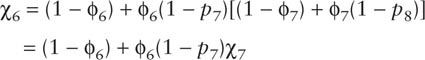
In fact, χi for any j can be calculated in the same way using the general recursive formula
![]()
Now suppose that eight samples are taken and the capture histories

are obtained for 14 animals. Suppose further that it is assumed that the probability of survival was constant during the study and that the probability of capture was constant for all samples. If Pi is the probability of capture history i occurring under the CJS model, then the full log likelihood for this set of capture histories is the sum of ln(Pi) for i = 1 to 14, i.e., ln(L) = ∑ln(Pi). If the constant probability of survival parameter is 0.6 and the constant probability of capture parameter is 0.2, then the log likelihood for this set of data could be calculated by setting ϕ1 = ϕ2 = … = ϕ8 = 0.6 and p2 = p3 = … = p8 = 0.2 in the CJS expression for Pj, taking the logarithms, and summing. If these calculations are carried out then it is found that ln(L) = −37.94. If the probability of survival were changed to 0.65 and probability of capture changed to 0.25, then ln(L) = −35.18. According to the theory of maximum likelihood, the parameters ϕ = 0.65 and p = 0.25 have a higher likelihood and are therefore better than the parameters ϕ = 0.60 and p = 0.20.

Figure 1.3. The full likelihood surface for the example with eight sample times and information on the captures and recaptures of 14 animals.
A computer can be programmed to repeatedly improve estimates of the parameters until ln(L) reaches a point where it cannot be increased further. For example, the SOLVER routine in Microsoft Excel can be used for this purpose providing that the likelihood function is not too complicated. With the example set of data, ln(L) will eventually reach a maximum of −32.60 when the survival parameter is ϕ = 0.78 and the capture probability parameter is p = 0.35. Because this example involves only two parameters, the entire likelihood surface is easy to plot and visualize, as shown in figure 1.3.
It is also possible to estimate the standard errors of parameter estimates from the likelihood function. The mathematical details justifying these estimates involve the second derivatives of ln(L), and will not be covered here. It suffices to say that the curvature of the likelihood provides some indication about the variance of the maximum likelihood estimate. For example, figure 1.3 shows that the likelihood is relatively flat for ϕ between 0.4 and 0.9, and p between 0.15 and 0.6. It can therefore be argued that any set of parameters in this flat region of the likelihood is reasonable. In general, if the likelihood has a flat region that is large, then the maximum likelihood estimates have large variances, but if the likelihood does not have a flat region, or the flat region is small, then the maximum likelihood estimates have small variances.
1.4 Model Selection Procedures
With the flexible modeling procedures that have become possible in recent years there has been a considerable increase in the number of models that can be considered for data sets with many sampling occasions. For example, with an open population it is often the case that capture and survival probabilities can be allowed to vary with time, the sex of the animal, weather conditions, etc. The problem is then to choose a model that gives an adequate representation of the data without having more parameters than are really needed.
There are two results that may be particularly useful in this respect. First, suppose that two alternative models are being considered for a set of data. Model 1 has I estimated parameters, and a log-likelihood function of ln(L1) when it is evaluated with the maximum likelihood estimates of the parameters. Model 2 is a generalization of model 1, with the I estimated parameters of model 1 and another J estimated parameters as well, and it has a log-likelihood function of ln(L2) when evaluated with the maximum likelihood estimates of the parameters. Because model 2 is more general (e.g., more complex) than model 1, it will be the case that ln(L2) is less than or equal to ln(L1). However, if in fact the extra J parameters in model 2 are not needed and have true values of zero, then the reduction in the log likelihood in moving from model 1 to model 2,
![]()
will approximate a random value from a chi-squared distribution with J degrees of freedom. Consequently, if D, the difference or deviance, is significantly large in comparison with values from the chi-squared distribution, then this suggests that the more general model 2 is needed to properly describe the data. If, on the other hand, D is not significantly large, then this suggests that the simpler model 1 is appropriate.
A limitation with the test just described is that it applies only to nested models, that is, where one model is a special case or subset of another model. This has led to the adoption of alternative approaches to model selection that are based on Akaike’s information criterion (AIC) (Akaike 1973; Burnham and Anderson 1998).
In its simplest form, AIC model selection involves defining a set of models that are candidates for being chosen as the most suitable for the data. Each model is then fitted to the data and its corresponding value for
![]()
is obtained, where L is the maximized likelihood for the model, and P is the number of estimated parameters. The model with the smallest value for AIC is then considered to be the “best” in terms of a compromise between the goodness of fit of the model and the number of parameters that need to be estimated. The balancing of model fit and number of parameters in the model is important in determining the precision of the estimates derived.
A further comparison between models can be based on calculating Akaike weights (Buckland et al. 1997). If there are M candidate models then the weight for model i is
![]()
where Δi is the difference between the AIC value for model i and the smallest AIC value for all models. The Akaike weights calculated in this way are used to measure the strength of the evidence in favor of each of the models, with a large weight indicating high evidence.
There are some variations of AIC that may be useful under certain conditions. In particular, for small samples (less than 40 observations per parameter) a corrected AIC can be used, which is
![]()
where n is the number of observations and P is the number of estimated parameters. Also, if there is evidence that the data display more variation than expected based on the probability model being used then this can be allowed for using the quasi-AIC values
![]()
where ĉ is an estimate of the ratio of the observed amount variation in the data to the amount of variation expected from the probability model being assumed, as explained more fully in chapter 9. The method for obtaining the estimate ĉ depends on the particular circumstances. When more variation than expected under a certain model is displayed, the data are said to be “overdispersed.” Overdispersion can arise in a number of ways. The most common causes are model misspecification (lack of fit) and a lack of true independence among observations. For example, the statistical likelihood for a set of capture data may assume that capture histories follow a multinomial distribution with a particular set of probabilities. If there is more variation in the capture histories than predicted by the multinomial distribution, the probabilities assumed in the multinomial model are incorrect, implying that the covariate model is misspecified, or there may be unaccounted for dependencies among the histories. In some but not all cases, apparent overdispersion can be remedied by incorporating more or different covariates into the model. Often, however, it will not be possible to account for some amount of overdispersion in the data.
1.5 Notation
A good deal of notation is necessary for describing the models used in the remainder of this book. The variation in notation can be quite confusing, particularly if sections of the book are read in isolation. To help reduce this confusion, all authors have standardized their notations, to the maximum extent practicable. In table 1.1 we have provided a summary of most of the notation used in the volume.
TABLE 1.1
Partial list of notation used throughout the book
Symbol |
Definition |
i |
An index for individual animals. Example: hi denotes the capture history for the ith animal. |
j |
An index for capture occasions (sample times). Example: pj is the probability of capture for the jth sample. |
k |
The number of capture occasions (samples) |
N |
A population size |
R |
A number of animals released |
m or n |
The number of animals with a certain characteristic. Examples: mh is the number of animals with capture history h, and nj is the number of animals captured in sample j. |
h |
A capture history. example: h = 001010. |
ϕ |
An apparent survival probability |
p |
A capture probability |
γ |
A seniority probability |
E |
A probability of emigration |
χ |
The probability of not being seen after a trapping occasion |
ξ |
The probability of not being seen before a trapping occasion |
M |
The number of marked animals in the population |
S |
A pure survival probability (not involving the probability of emigration); also, the number of strata in a multistrata model |
F |
A probability of not emigrating, equal to 1 − E. |
R |
A reporting probability |
ρ |
A resighting probability |
F |
A tag recovery probability, equal to r(1 − S) when there is no emigration |
ψ |
A probability of moving between strata from one sampling occasion to the next for a multistrata model |
Note. In some cases, symbols not listed here may be defined to represent different things in different chapters. For example, in chapter 6 S represents a pure survival probability that does not include probability of emigration, while in chapter 8 S represents the number of strata in a multistrata model. These cases have been kept to a minimum and the meaning of each symbol is clear from the context. Symbols listed here can be subscripted or superscripted as needed. For example, Ni might denote the sample size at the time of the ith sample time. Also, a caret is often used to indicate an estimate, so that |
|

Figure 1.4. Black bear (Ursus americanus), near Council, Idaho, 1973, wearing numbered monel metal ear tags. (Photo by Steven C. Amstrup)