Five

Modern Open-population Capture–Recapture Models

JAMES D. NICHOLS

5.1 Introduction

Capture–recapture studies of open populations involve multiple sample occasions at which newly captured animals are individually marked and identities of previously captured animals are recorded. Sample occasions are separated by time intervals that are sufficiently large that the population is expected to change between occasions. Hence, the population is said to be open to gains resulting from in situ reproduction and immigration and to losses from death and emigration.

Two classes of models have been developed to estimate quantities of interest from the data resulting from studies of open populations. The first class can be referred to as conditional and is exemplified by the original model of Cormack (1964; chapter 3 in this volume). This modeling is conditional on the number of animals released at each sampling occasion and permits estimation of subsequent survival and capture probabilities. The second class is unconditional and is exemplified by the models of Jolly (1965) and Seber (1965). This approach models not only the history of marked animals following release, but also the initial captures of unmarked animals, permitting estimation of such quantities as abundance, recruitment, and rate of population change.

In addition to these two approaches for modeling data from open populations, Pollock (1982) introduced a robust design that involves sampling at two temporal scales. Primary sampling periods are separated by relatively long periods, and the modeling of capture histories over these periods is based on models for open populations. However, within each primary sampling period, there are multiple secondary sampling periods separated by relatively short time intervals. The capture histories over these secondary periods are typically modeled using models for closed populations (Otis et al. 1978).

Figure 5.1. A leg-banded female Canada goose (Branta canadensis) defends her nest near Anchorage, Alaska. Checking nests to resight marked individuals, which are usually faithful to nesting areas, allows the estimation of the annual survival rate. (Photo by Jerry Hupp)

5.2 Conditional Single-age Models

Whereas chapter 3 provided closed-form estimators that can be computed as functions of summary statistics, this chapter focuses on models that are generally implemented using iterative techniques based on individual capture histories. A capture history (chapter 1) is simply a list of 1’s and 0’s, where 1 indicates that the animal was caught or observed, and 0 indicates that the animal in question was not caught or observed. For example, the capture history 01010 indicates an animal that was caught on the second and fourth sampling occasions of a 5-occasion study but not on occasions 1, 3, or 5. Every animal caught at least once during a study has a known capture history, and these data can be summarized as the number of animals exhibiting each history. For example, x₀₁₀₁₀ indicates the number of animals in the study exhibiting the history 01010.

capture–recapture estimation is based on probabilistic models for events that give rise to a capture history. Conditional Cormack-Jolly-Seber (CJS) (Cormack 1964; Jolly 1965; Seber 1965) modeling of capture–recapture data for open populations is based on two primary parameters:

p_j = the probability that a marked animal in the study population at sampling period j is captured or observed during period j; and

ϕ_j = the probability that a marked animal in the study population at sampling period j survives until period j + 1 and remains in the population (i.e., the animal does not die or permanently emigrate).

In addition,

χ_j = the probability that an animal alive and in the study population at sampling period j is not caught or observed again at any sampling period after period j.

For a capture–recapture study with k sampling periods χk = 1, and values for sampling period j < k can be computed recursively as

x_j = (1 – ϕ_j) + ϕ_j(1 – p_{j + 1})χ_{j + 1}

Thus, χ_j is not really a new parameter but simply a function of the two primary parameters.

As explained in chapter 1, the modeling process can be illustrated by writing the probability corresponding to the example capture history 01010 as

Pr(01010 | release in period 2) = ϕ₂(1 – p₃)ϕ₃p₄χ₄

As the modeling approach conditions on the initial release, there are no parameters associated with capture in periods 1 or 2. However, the animal survived from period 2 to 3, and the probability associated with this event is ϕ₂. It was not captured in period 3, and the corresponding probability is given by (1 − p₃); it survived from 3 to 4 (ϕ₃) and was caught (p₄), and finally it was not caught again after 4 (χ₄ = 1 – ϕ₄p₅).

Note that the above modeling would differ slightly if the animal died in a trap or was otherwise removed from the population in period 4. In this case, the capture history would be modeled as

Pr(01010 | release in period 2 and removal at period 4) = ϕ₂(1 − p₃)ϕ₃p₄

The χ₄ term is no longer appropriate as the final entry, because the animal is not exposed to survival and capture probabilities following period 4.

The complete likelihood for the CJS model can be written as the product of the probabilities associated with each capture history, conditional on the initial capture and release of each animal (Seber 1982; Lebreton et al. 1992). The result is a product-multinomial likelihood (a likelihood function resulting from multiplying more than one likelihood function, see chapter 1) that specifies a probability for each possible capture history given the number of animals exhibiting each capture history. Maximum likelihood estimation can then be used to obtain estimates of the model parameters, ϕ_j and p_j. Under the CJS model all parameters are time-specific. It is not possible to estimate the initial capture probability, p₁, and the final survival and capture probability of a study cannot be estimated separately, but only as a product ϕ_{k − 1}p_k.

The following assumptions typically are listed for the CJS model (e.g., Seber 1982; Pollock et al. 1990):

1. every marked animal present in the population at sampling period j has the same probability p_j of being recaptured or resighted;

2. every marked animal present in the population immediately following the sampling in period j has the same probability ϕ_j of survival until sampling period j + 1;

3. marks are neither lost nor overlooked, and are recorded correctly;

4. sampling periods are instantaneous (in reality they are very short periods) and recaptured animals are released immediately;

5. all emigration from the sampled area is permanent; and

6. the fate of each animal with respect to capture and survival is in dependent of the fate of any other animal.

 

Consequences of violating these assumptions have been well studied and are summarized in chapter 3 (also see Seber 1982, pp. 223–232; Pollock et al. 1990; Williams et al. 2002, pp. 434–436).

Substantial attention has been devoted in the literature to assumptions 1 and 2, which concern homogeneity of the rate parameters that underlie the capture-history data. Survival and capture probabilities frequently vary as a function of the attributes of a captured or observed animal. Much work in capture–recapture modeling over the last two decades has involved efforts to model variation in survival and capture parameters as functions of variables characterizing the state of individual animals at different times (e.g., Lebreton et al. 1992; Nichols et al. 1994).

Reduced-parameter Models

The CJS model yields closed-form estimators that are readily computed (chapter 3, this volume) and was virtually the only model used for estimating survival rates from capture–recapture data for the first 15–20 years following its development. However, with a separate parameter for capture and survival probability for each sampling period, the model was more general than needed in many cases, and this often resulted in estimates with large variances. As access to computers increased, statisticians began to consider reduced-parameter models that required iterative solutions to obtain parameter estimates (e.g., Cormack 1981; Sandland and Kirkwood 1981; Jolly 1982; Clobert et al. 1985; Crosbie and Manly 1985). As noted in chapter 3, the initial reduced-parameter models constrained either capture probability or survival probability or both parameters to be constant over time (i.e., p_j = p and ϕ_j = ϕ).

In the event of unequal time intervals between sampling occasions, the constraint ϕ_j = ϕ is not likely to be reasonable (i.e., survival probabilities will tend to be smaller for longer time intervals). In this case a more reasonable constraint would be for survival per unit time to be a constant, so that ϕ_j = ϕ^tj, where t_j is the number of time units separating sampling occasions j and j+ 1, and ϕ is the survival probability per unit time (Brownie et al. 1986).

The likelihoods for reduced-parameter models are created by substituting the single, time-constant parameter for the corresponding time-specific parameter in the CJS likelihood (e.g., p for p_j). Maximum likelihood estimation can then be conducted numerically (e.g., section 1.3; White and Burnham 1999), as closed-form estimators are not available. Likelihood ratio tests can be used to test between competing models (Lebreton et al. 1992), or information-theoretic approaches such as Akaike’s Information Criterion (AIC) can be used to select the appropriate model from a set of candidate models (chapter 1; Akaike 1973; Anderson et al. 1994; Burnham and Anderson 1998).

Time-specific Covariates

In many situations, survival and capture probabilities can be modeled as functions of time-specific external variables. For example, environmental variables might influence either capture or survival probabilities, or variables reflecting sampling effort might be related to capture probabilities. Such modeling involves incorporation of the hypothesized covariate model directly into the likelihood (North and Morgan 1979; Clobert and Lebreton 1985; Clobert et al. 1987; Lebreton et al. 1992), and maximum likelihood estimation can then be used to estimate the parameters of the functional relationship directly.

Lebreton et al. (1992) considered the use of a link function (McCullagh and Nelder 1989), a function f that links the parameter of interest to a (typically) linear function of (possibly) multiple covariates; for example, f(x_gj), where x_gj denotes the value of covariate g at sampling occasion j, and the β_g are parameters associated with this relationship. The link function is also often expressed using its inverse, f⁻¹. Link functions noted as potentially useful by Lebreton et al. (1992) include the identity function f⁻¹(x) = x, the logit function f⁻¹(x) = logit(x) = ln[x/(1 − x)], the logarithm function f⁻¹(x) = ln(x), and the hazard function f⁻¹(x) = ln[−ln(x)].

The logit link function is used frequently in capture–recapture modeling and associated software (e.g., White and Burnham 1999) and has the advantages of providing a flexible form and bounded estimates for ϕ_j and p_j in the interval (0,1). For example, modeling of survival using the logit link essentially substitutes the following model for ϕ_j in the likelihood function:

Maximum likelihood estimates of the β parameters can then be obtained numerically via maximization of the likelihood function, using iterative methods as described in chapter 1.

Multiple Groups

capture–recapture data sometimes can be grouped into distinct cohorts. For example, both males and females are captured in many studies, and it is often reasonable to suspect that the sexes do not have equal survival and recapture probabilities. One approach to parameter estimation would be to use completely different parameters to model the capture histories for the two sexes, estimating sex-specific survival and capture probabilities. For example, a three-period study would include the following parameters: , where the superscript denotes the sex (1 = male and 2 = female). Note that because the CJS and related models are conditional on the initial capture (modeling involves only subsequent events in the capture history), the above set of parameters does not include the capture probabilities for the first sampling period . Also note that all of the above parameters cannot be separately estimated. In particular, under the CJS model, the final capture and survival probabilities cannot be estimated separately but only as a product (ϕ_{k − 1} p_k). Thus, although the example three-period model contains 8 parameters, only 6 can be estimated: . Such a model is generally denoted as model (ϕ_s*t, p_s*t), where the model notation subscripts s and t denote sex and time, respectively. The asterisk indicates that if the model is written as a generalized linear model (McCullagh and Nelder 1989), it includes parameters for all interaction terms between the different levels of the associated factors s and t. For example, survival probabilities for the above three-period model can be written as

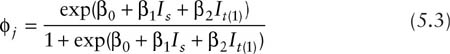
where β₀ is an overall intercept term, β₁ is a parameter associated with sex with I_s = 1 for males and 0 for females, β₂ is a parameter associated with the first sampling period 1 with I_t(1) = 1 when j = 1 and 0 otherwise, and β₃ is an interaction parameter associated with males in the first sampling period with I_s = 1 and I_t(1) = 1. Note that the survival model of equation (5.2) contains four parameters, as was also the case when we used a different survival parameter for each possible sex-time combination. These are simply two different ways of writing the same model.

In the case of general model (ϕ_s*t, p_s*t), none of the original parameters are the same for the two sexes. However, there are many situations in which either survival or capture probabilities or both should be similar for the two sexes. Such models can be constructed by imposing constraints on the general model. For example, the model (ϕ_s*t, p_t) includes different time-specific survival probabilities for males and females, yet assumes common capture probabilities for the sexes. In the above example with three sample periods, the total number of parameters (ignoring estimability questions) is reduced from 8 in the full model to 6 in model (ϕ_s*t, p_t).

A useful class of constraints for multiple groups involves the idea of parallelism (Lebreton et al. 1992), which links the temporal variation in a parameter for two or more groups. For example, Lebreton et al. (1992) use the notation (ϕ_s+t, p_s*t), to denote a model with time specificity and sex specificity of both survival and capture probability parameters, with the s + t notation of the survival parameter indicating that survival varies over time, but does so in a parallel or additive manner for the two sexes. One way to write this model is to simply remove the interaction parameter from the full model of equation 5.2 to yield the parallel parameterization

The number of parameters is reduced by only one (from four to three) in this example, but in cases with moderate to large numbers of sample periods, the reduction can be substantial.

Finally, note that the modeling of multiple groups is very general and can include animals at multiple locations or perhaps exposed to multiple experimental treatments. Modeling of such data would then focus on the possible existence of spatial variation or treatment-induced variation, respectively, in the parameters of interest.

Effects of Capture History

As noted above, the CJS model assumes that all marked animals present in the population during sampling period j have equal probabilities of being caught (or resighted) that time, and of surviving to any subsequent sampling period. Robson (1969) and Pollock (1975) first considered more general models in which individuals alive in the sampled population at period j could exhibit different capture and survival probabilities at period j depending on their previous capture history.

A useful example of capture-history dependence involves trap response in capture probabilities (Cormack 1981; Sandland and Kirkwood 1981; Lebreton et al. 1992; Pradel 1993). Sandland and Kirkwood (1981) considered a simple model of trap dependence with different capture probabilities for an animal at period j, depending on whether or not the animal had been captured at period j − 1. That is,

p_j = the capture probability at sampling period j for an animal that was caught at j – 1; and

= the capture probability at sampling period j for an animal that was not caught at j – 1.

Sandland and Kirkwood (1981) obtained estimates under a reduced-parameter version of the above model in which the capture probabilities were constant over time, but survival probabilities were time dependent. Under this model, the subscript j is dropped so that p_j = p and = p′.

To illustrate this parameterization, consider the probability of observing the following capture history 01010 under the above trap-dependence model of Sandland and Kirkwood (1981):

Pr(01010 | release in period 2) = ϕ₂(1 – p)ϕ₃p′(1 – ϕ₄p)

The capture probability parameters associated with sampling periods 3 and 5 correspond to animals caught the previous time periods (2 and 4, respectively), whereas the capture probability for period 4 corresponds to an animal not caught the previous period.

Trap response can also occur in survival, such that survival between periods j and j + 1 depends on capture history before and including period j. For example, Brownie and Robson (1983) considered the sampling situation in which a mark is applied at initial capture, and subsequent encounters with marked animals are resightings. If trapping or handling adversely affects survival, then such an effect most likely occurs during the interval immediately following capture (the initial encounter). Brownie and Robson (1983) thus parameterized survival as

ϕ_j = the probability that a previously marked animal in the sampled population at time j survives until time j + 1 and remains in the sampled population; and

= the probability that a previously unmarked animal in the sampled population at time j survives until time j + 1 and remains in the sampled population.

As an illustration of the parameterization under the Brownie-Robson (1983) model, consider the capture history and associated probability

The survival probability following release in period 2 includes the prime notation because it corresponds to an animal that has not been previously marked, whereas the subsequent survival parameters correspond to resightings of marked animals. Both kinds of survival parameters can be written as linear-logistic functions of covariates as in equation 5.1.

Pradel et al. (1997a) reparameterized the Brownie-Robson (1983) model to correspond to the situation in which unmarked animals are viewed as being of two groups, residents that have a chance of surviving and being recaptured, and transients that are just moving through the study area and have no chance of being seen again on the area. The presence of transients (with apparent survival probability of 0) among unmarked animals causes the survival probability of new animals to be lower than that of marked animals (these are residents by definition). The parameterization of Pradel et al. (1997a) thus permits estimation of resident survival probability as well as the probability that an unmarked animal is a transient.

Individual Covariates

The CJS model and the models derived from it assume homogeneity of capture and survival probabilities among individuals at some level of grouping. For example, even in the case of dependence on previous capture history, homogeneity is assumed to apply to all animals with a particular history. Of course, strict homogeneity (exact equality) of survival and capture probabilities of different individual animals is unlikely ever to be true, regardless of the manner in which animals are grouped or categorized. Sometimes a substantial amount of variation among individuals in survival and capture probabilities may be explained by a single measurable covariate, for example: size or weight at some critical stage in the early life of an animal, mass at hatch or fledging (Perrins 1963, 1965), or parental size and experience (Hastings and Testa 1998).

Individual covariates of this type are static, in the sense that the single measurement characterizes the animal throughout the capture–recapture study (perhaps throughout life). Individual-based modeling is based on the view that the capture history of each individual animal is a multinomial sample with sample size of 1 (Smith et al. 1994). The full development of individual-based modeling is presented by Skalski et al. (1993), Smith et al. (1994), and Hoffman and Skalski (1995). An important point is that such modeling can be implemented in software such as SURPH (Smith et al. 1994) and MARK (White and Burnham 1999). As with multiple groups and time-specific covariates described above, link functions (e.g., logit or hazard) are used to model the individual survival or capture probabilities as functions of individual-level covariates, as well as group-specific and time-specific covariates.

We emphasize that these individual covariate models assume that the covariate characterizes the animal throughout the study. Time-varying individual covariates cannot be measured for animals that are not caught in a sampling period and thus cannot be used to model survival or capture probabilities. Such modeling requires models for the change in the covariate over time, and this is both reasonable and possible in some sampling situations (S. Bonner and C. Schwarz, personal communication). However, at present, use of time-varying individual covariates is most readily accomplished with existing software via discretization into groups and use of multistate models (Nichols et al. 1992b; chapter 8).

Model Selection and Related Issues

The large number of potential models, even for the single-age situation, emphasizes the need for a reasonable approach to model selection. Under one reasonable approach, the investigator begins with an a priori model set and must then decide which model(s) is best supported by the data, in the sense of adequately describing variation in the data in a parsimonious manner (without too many parameters). As noted in chapter 1, AIC (Akaike 1973) has been recommended for this purpose (e.g., Anderson et al. 1994; Burnham and Anderson 1992, 1998, 2002). Use of AIC presupposes that at least one model in the model set provides a reasonable fit to the data. Thus, a useful first step is to conduct a goodness-of-fit test of the most general model in the model set.

Goodness-of-fit tests have been developed specifically for the CJS model (Pollock et al. 1985, implemented in program JOLLY; Burnham et al. 1987, implemented in program RELEASE), and the Brownie-Robson trap response model (Brownie and Robson 1983, implemented in program JOLLY), for example. The CJS model tests of Pollock et al. (1985) and Burnham et al. (1987) have the same basic structure and differ only in their method of pooling of data. The CJS model test implemented in program RELEASE is labeled as the sum of two sets of contingency table tests, TEST 2, which focuses on subsequent capture histories of animals in different release cohorts, and TEST 3, which focuses on subsequent capture histories of animals within each release cohort, but with different prior histories (Burnham et al. 1987). The TEST 2 + TEST 3 sum is distributed as χ² under the null hypothesis of reasonable model fit. If it is judged to be significant, then the test statistic can be used to compute a variance inflation factor as

where df is the degrees of freedom associated with χ² test statistic. Note that under the null hypothesis of reasonable model fit

so that

For other models without well-developed goodness-of-fit tests, a Pearson goodness-of-fit test can often be computed. However, in many cases these tests do not perform well when a large proportion of contingency table cells must be pooled because of sparse data and low expected cell values. An alternative means of assessing fit is based on a parametric bootstrap approach that can be implemented using program MARK (White et al. 2001). This method uses the estimates for the model of interest, which is frequently the most general model in the model set. The estimates from this model for the real data are assumed to be good approximations for the true parameter values, and many new data sets are generated by simulation using the model with the estimated parameter values. The assumed model is fitted to each of the generated sets of data, and the deviance is computed. The observed deviance from the actual capture history data set can then be compared with the generated distribution of deviances to assess fit.

This then yields two approaches for estimating ĉ (White et al. 2001). Under the first approach, it is estimated as the observed deviance divided by the mean of the bootstrap deviances, as this latter mean should estimate the deviance in the case where the model fits the data adequately. The second approach uses the observed ĉ (computed as the deviance divided by the model df) divided by the mean of the deviance/df from the bootstrap iterations. These two approaches give different results because the df for a set of data varies from one generated data set to the next with parametric bootstrapping. Neither of the approaches works well in all situations, and goodness of fit is an important issue requiring additional work in open capture–recapture modeling.

Most of the theory underlying use of such a variance inflation factor is based on the assumption that overdispersion is the source of the lack of fit, but the ĉ factor is used more widely, as the true reasons underlying a lack of fit are seldom known. In the case of overdispersion, a model-based variance estimate vâr() will typically be too small and should be modified to ĉ vâr().

If even the most general model in the set does not appear to fit the data well, then a quasilikelihood approach is recommended for both likelihood ratio testing and model selection (Burnham et al. 1987; Mc-Cullagh and Nelder 1989; Lebreton et al. 1992; Burnham and Anderson 2002, chapter 1). In the case of overdispersion, likelihood ratio tests can be modified using ĉ to yield F statistics for testing between nested models (Lebreton et al. 1992). In the case of lack of fit, or when ĉ > 1, the AIC model selection statistic can be modified to

where L() is the likelihood function evaluated at the MLEs of the parameters, and K is the number of parameters in the model, plus one parameter corresponding to ĉ (Burnham and Anderson 2002). In addition to this quasilikelihood adjustment, most general capture–recapture models have large numbers of parameters to be estimated from relatively small samples, leading to an AIC statistic adjusted for both quasi-likelihood and small sample size:

where n denotes the effective sample size. The sample size is not so easily defined in capture–recapture modeling, and Burnham and Anderson (2002) suggest use of the number of distinct animals captured once or more.

Model selection proceeds using ranked AIC or QAIC_c values, with the model exhibiting the lowest value selected as the most appropriate for the data. Model ranks based on this selection process are typically expressed as ΔAIC_i, or simply as Δ_i, computed as the difference between the AIC statistic for model i and the model with minimum AIC. These Δ_i can then be used to compute model-specific AIC weights:

where the summation is over all of the models in the model set. These weights reflect the proportional support or weight of evidence for a specific model (Burnham and Anderson 2002). If several models exhibit similar AIC values, then weighted estimates of important parameters can be obtained as a weighted mean of estimates from multiple models, with each model’s estimate being weighted by its AIC weight (Buckland et al. 1997; Burnham and Anderson 2002).

Example

Methods for single-age capture–recapture analysis are illustrated here with a live-trapping study of meadow voles, Microtus pennsylvanicus, at the Patuxent Wildlife Research Center, Laurel, MD. Details of trapping and field methods are provided by Nichols et al. (1984b). Although trapping was conducted under the robust design (Pollock 1982), the five days of sampling in each month were collapsed into a single assessment of whether each animal was caught at least once, or not, for each of the six monthly sampling occasions. Resulting capture history data are presented in table 5.1. Note that a small number of animals was lost on capture because they died in the trap.

TABLE 5.1
Adult capture history data for a six-period study of meadow voles, Microtus pennsylvanicus, at Patuxent Wildlife Research Center, Laurel, Maryland, 1981

TABLE 5.2
Parameter estimates under the general two-sex CJS model (ϕ_s*t, p_s*t) for adult meadow voles studied at Patuxent Wildlife Research Center, Laurel, Maryland, 1981

The most general model considered (ϕ_s*t, p_s*t) for fitting to the data represents a combination of separate CJS models for the two sexes. The fit of this model to the data was judged to be adequate (, P = 0.14) based on the overall goodness-of-fit test of program RELEASE (Burnham et al. 1987). The high capture probability estimates under this model reflect the five days of trapping, and the monthly survival estimates are typical of meadow voles (table 5.2).

A number of reduced-parameter models were also fitted to these data. For a full analysis see Williams et al. (2002, pp. 436–439). Several of these models were judged to be more appropriate than (ϕ_s*t, p_s*t). The general model (ϕ_s*t, p_s*t) showed ÄAIC_c = 5.25 relative to the low-AIC_c model, (ϕ_s+t, p). Under the low-AIC_c model (ϕ_{s + t}, p), survival probability varied by sex and time, but the temporal variation was parallel (on a logit scale) for the two sexes (figure 5.2), with survival for females slightly higher than that for males. The capture probability was best modeled using a single value that was constant over time and the same for both sexes.

5.3 Conditional Multiple-age Models

In addition to the models described above, one way to relax the CJS assumption of homogeneous capture and survival probabilities is to permit age-specific variation. There are three classes of age-specific models that differ in the data structures for which they were developed.

Figure 5.2. Estimated monthly survival probabilities and 95% confidence intervals from model (ϕ_{s + t}, p) for male and female meadow voles at Patuxent Wildlife Research Center.

Pollock’s Multiple-age Model

This model was developed by Pollock (1981b); also see Stokes (1984). It assumes the existence of I + 1 age classes (0, 1, . . . , I) that can be distinguished for newly caught (unmarked) animals, with age class I including all animals of at least age I. The model requires a design restriction that the timing of sampling and age class transition are synchronized, such that an individual of age υ in sample period j will be at age υ + 1 in sample period j + 1. Here, we discuss the simplest case in which I = 1, with young (υ = 0) and adults (υ = 1) as the distinguishable age classes. Estimation under the Pollock (1981b) model is based on the numbers of animals in each age class exhibiting each of the observable capture histories (denoted by for capture history ω and age υ, where υ corresponds to the age at initial capture). For example, is the number of animals released as young in period 2 and recaptured (as adults) in period 3.

Parameters are defined in a manner similar to the single-age case, with the additional notation of a superscript denoting age:

= the probability that a marked animal of age υ in the study population at sampling period j is captured or observed during period j;

= the probability that a marked animal of age υ in the study population at sampling period j survives until period j + 1 (to age υ + 1) and remains in the population (does not permanently emigrate); and

= the probability that an animal of age υ in the study population at sampling period j is not caught or observed again at any sampling period after period j. As in the case of single-age models, the parameters are written as functions of and parameters. In the two-age case, for example, is defined just as in the CJS model using all adult parameters, and can be written as

The modeling of capture-history data proceeds in the same manner as with the single-age CJS model. Consider capture history 01010 for animals marked in period 2. Modeling of this history is again conditional on the initial capture at period 2 and is dependent on the age of initial marking. In the 2-age situation,

These probabilities differ only in the superscript of the initial survival probability. Animals initially released as young survive the interval following initial release (periods 2–3) with a survival parameter associated with young animals. But subsequent capture and survival probabilities correspond to adult animals, as the young animal in period 2 makes the transition to the adult class in the interval between periods 2 and 3. As with single-age models, if the animal is removed (not released) following the last capture, then the final term is simply removed from the capture history model. Age-specific modeling of survival can also be accomplished by writing the logit of survival as a linear function of age in the same way as was done for sex, i.e., by substituting I_a (1 for adults and 0 for young) for I_s, and I_a(tj) for I_s(tj) in equation 5.2. As was the case for the additive modeling of sex and time effects, deletion of the interaction terms results in a model in which survival differs for the different ages but is parallel (on a logit scale) over time.

The complete likelihood for the Pollock (1981b) multiple-age model can be written as a product-multinomial likelihood that specifies a probability for each possible capture history together with the actual data, the number of animals exhibiting each capture history. Maximum likelihood estimation can then be used to obtain estimates of the model parameters, and .

Model assumptions are very similar to those listed for the single-age CJS model. Assumptions 1 and 2 of the CJS model are modified for the age-specific model to restrict homogeneity of capture () and survival () probabilities to members of the same age class (υ) at each sampling period (e.g., survival probability must be the same for all animals of age υ but not for animals of different age classes). The age-specific models of Pollock (1981b), Stokes (1984), and Brownie et al. (1986) also assume that age is correctly assigned to each new animal that is encountered and marked.

Reduced-parameter models were presented for multiple age classes by Brownie et al. (1986) and Clobert et al. (1987), and are also described in Pollock et al. (1990) and Lebreton et al. (1992). Reduced-parameter models of interest include those constraining parameters to be constant over time, as well as models constraining parameters to be constant across age classes. Time-specific and individual covariate models can be developed for multiple ages following the same general principles outlined for single-age models. Models with multiple groups and capture-history dependence are also developed for multiple ages in the same manner as for a single age. Estimation under these various models can be carried out by program MARK (White and Burnham 1999). Finally, the general principles of model selection described for single-age models are also applicable to multiple ages. Goodness-of-fit tests for the Pollock (1981b) and reduced-parameter models were developed by Brownie et al. (1986); also see Pollock et al. (1990).

Age 0 Cohort Models

It is also possible to focus on cohorts of animals released as newborns (age 0) in situations where the age of organisms can be distinguished only in terms of young (age 0) and older (age >0) individuals. The only way to know the specific age of an adult animal is for the animal to have been released in a previous period at age 0. New, unmarked adults are thus not used in the modeling. The development of these models assumes that the interval between sampling occasions coincides with the time period required for the animals to mature from one age class into the next (e.g., annual sampling with year age classes). The notation for capture-history data is the same as that for the Pollock (1981b) model. With the cohort model, however, all animals used for modeling are marked as young (υ = 0), so all capture-history statistics are superscripted with (0). Cohort models also have been used for unaged adults (Loery et al. 1987). In such cases, the superscript for both data and parameters corresponds to the number of time periods since initial capture rather than to age. This notation highlights the operational definition of cohort in the context of these models as a group of animals initially captured at the same occasion and, in some cases, of the same age.

Models for cohort data were considered by Buckland (1980, 1982), Loery et al. (1987), and Pollock et al. (1990). Notation is similar to that of the age-specific models of Pollock (1981b), with probabilities of capture () and survival (). Modeling is also similar to that for the Pollock (1981b) models, except that age is defined not only for classes recognizable at capture but for animals of all ages, given that they were initially caught at age υ = 0. For example, the probability associated with capture history 01010 for individuals first captured as young in year 2 is

Every increase in sample period (subscript j) is accompanied by an increase in age (superscript υ). This general cohort model can be viewed as a series of separate CJS models, one model for each cohort of age-0 releases. Age-0 cohort models and various derivative models (e.g., reduced-parameter, covariates, multiple groups) can be implemented in MARK (White and Burnham 1999). This class of models can be used to address questions about senescent decline in survival probability (see Pugesek et al. 1995; Nichols et al. 1997). For such questions it is frequently useful to write the logit of age-specific survival rate as a linear function of age.

Age-specific Breeding Models

Not all ages are exposed to sampling efforts under some capture–recapture sampling designs. Young of many colonial breeding bird species depart the breeding ground of origin following fledging and do not return to the breeding colony of origin until they are ready to breed. Thus, prebreeders of age >0 can be viewed as temporary emigrants with probability 0 of being captured or observed prior to their first breeding attempt. Temporary emigration of this sort can be dealt with using either the robust design (see section 5.6) or standard open-model capture history data modeled with a structure that accommodates the absence of prebreeders.

Using this latter approach, Rothery (1983) and Nichols et al. (1990) considered estimation in the situation where all birds begin breeding at the same age. Clobert et al. (1990, 1994) considered the more general situation where not all animals begin breeding at the same age. Clobert et al. (1994) describe a two-step approach in which age-specific breeding probabilities are estimated as functions of capture probabilities estimated from a cohort model. Spendelow et al. (2002) and Williams et al. (2002, pp. 447–454) used this idea to develop a model that estimates the probability that an animal of age υ that has not become a breeder before time j does so at time j. Although the general model has been used primarily for birds, it may be useful for a variety of other groups, including sea turtles, anadromous fish, some amphibians, and some marine mammals.

5.4 Reverse-time Models

The models discussed thus far are conditioned on numbers of releases at a given sampling period, and they describe the remainder of the capture history. Pollock et al. (1974) noted that if the capture-history data are considered in reverse time order, conditioning on animals caught in later time periods and observing their captures in earlier occasions, then inference can be made about the recruitment process. More recent uses of reverse-time capture–recapture modeling include Nichols et al. (1986, 1998), Pradel (1996), Pradel et al. (1997b) and Pradel and Lebreton (1999).

The data for reverse-time modeling are the same as previously described for forward-time modeling and consist of the numbers of animals exhibiting each observable capture history. The modeling is similar to that described above for the CJS model, the time direction being the only real difference. Two primary parameters are defined to be

γ_j = the probability that an animal present just before time j was present in the sampled population just after sampling at time j – 1, and

= the probability that an animal present just after sampling at time j was captured at j.

The parameters γ_j were termed “seniority” parameters by Pradel (1996). They can be viewed as survival probabilities that extend backward in time. Note that both the seniority and capture probabilities are defined carefully relative to the time of sampling (just before or after sampling). The reason for this attention to timing concerns losses on capture. For the discussion here, we will typically assume no losses on capture for ease of presentation. In this case, the capture probability parameters are identical for forward and reverse time modeling, = p_j.

In addition to the above parameters, let ξ_j be the probability of not being seen previous to time j for an animal present immediately before j.

The parameter ξ_j, which is analogous to χ_j in standard-time modeling, can be written recursively

for j = 2, 3, . . . , k, with ξ₁ = 1. To have not been seen before time j, an animal either must not be a survivor from time j – 1 (this possibility occurs with probability 1 – γ_j), or it must be a survivor (with probability γ_j) that was not caught in j – 1 (with probability 1 – − ₁) and not seen before j – 1 (with probability ξ_{j − 1}).

Consider the reverse-time modeling of capture history data, using the same history that was used to illustrate standard-time modeling. Again consider history 01010, indicating capture in periods 2 and 4 of a five-period study. For reverse-time modeling we condition on the final capture and model prior events in the capture history:

Beginning with the final capture in period 4 and working backward, the animal exhibiting this history was an old animal at 4, in the sense that it was a survivor from period 3. The associated probability is γ₄. The animal was not captured at time 3 (associated probability is 1 – ). It was a survivor from 2 (γ₃), and it was again caught at 2 (). However, it was not seen before period 2 (ξ₂). Note that unlike the case with standard-time modeling, the reverse-time capture history modeling does not differ depending on whether or not the animal was released following the final capture in the history. The reverse-time modeling only involves events occurring prior to this time.

Conditional multinomial models can be developed by conditioning on the number of animals caught for the last time at each period, j, and then using the numbers of these animals exhibiting each capture history, in conjunction with the probabilities associated with each history. Estimation of model parameters is accomplished using the method of maximum likelihood. In fact, estimates of γ_j and can be obtained by simply reversing the time order of capture-history data and obtaining estimates using software developed for standard-time analyses (Pradel 1996). Program MARK (White and Burnham 1999) contains a routine to provide estimates under reverse-time modeling.

The assumptions underlying reverse-time modeling are similar to those underlying standard-time models. The homogeneity assumptions (1, 2) now apply to the seniority and capture probabilities rather than to survival and capture probabilities. For reverse-time modeling, every marked and unmarked animal present in the population at sampling period j must have the same probability of being captured. This assumption can be restrictive and is important to recall when estimating γ_j.

The reverse-time parameters, γ_j, reflect the proportional change in population growth rate, λ_j, that would result from a specified proportional change in survival probability. The complement, 1 – γ_j, reflects the proportional change in λ_j that would result from a specified proportional change in recruitment of new animals. These parameters are thus analogous to the elasticities computed for projection matrix parameters (Caswell 2001). A discussion of the use and interpretation of reverse-time capture–recapture estimates is presented by Nichols et al. (2000). Combination of standard-time and reverse-time modeling in a single likelihood permits direct estimation of λ_j and is considered in section 5.5, as well as by Pradel (1996) and Nichols and Hines (2002).

The same kinds of modeling can be used with reverse-time capture–recapture as with standard time. Reduced parameter models and models with time-specific and individual covariates can be developed. Multiple age models can also be developed but require multistate models (Arna-son 1973; Hestbeck et al. 1991; Brownie et al. 1993; chapter 8) and a robust design approach (see Nichols et al. 2000).

5.5 Unconditional Models

Here, we consider the estimation of population size and recruitment using capture–recapture data for open (to gains and losses between sampling occasions) populations. We focus on single-age models, where we consider all animals as adults.

For standard capture–recapture sampling, the data collected are identical to those used for the conditional models described above, but there is increased emphasis on the number of unmarked animals in unconditional modeling. In standard capture–recapture studies, unmarked animals that are captured are given tags permitting individual identification, and the number of these animals is recorded. In capture-resighting studies, an effort must be made to count the number of unmarked animals encountered during the resighting sampling efforts. These counts of unmarked animals, which are not needed for survival rate estimation with conditional models, play a key role in estimation of population size and recruitment.

The Jolly-Seber (JS) Model

The JS model includes the CJS structure for modeling capture histories conditional on initial capture and release. The JS model also includes an additional component for modeling the number of unmarked animals caught in sampling period j (denote as u_j) as a function of the total number of unmarked animals, U_j, in the population, i.e., E(u_j | U_j) = p_jU_j.

The following are unknown random variables, the values of which are to be estimated:

N_j = the total number of animals in the population exposed to sampling efforts in sampling period j; and

B_j = the number of new animals joining the population between samples j and j + 1, and present at j + 1.

Jolly (1965) and Seber (1965) presented closed-form estimators of the above quantities, as discussed in chapter 3.

These estimators can be derived by obtaining maximum likelihood estimates of survival and capture probabilities using the conditional portion of the likelihood, which is the same as the entire CJS likelihood (Brownie et al. 1986; Williams et al. 2002), and then applying the resulting time-specific estimates of capture probability to the total number of animals caught in each sampling period. Thus, n_j = u_j + m_j, where m_j denotes the number of marked animals caught at j, and

Substitution of (where is the estimated number of marked animals in the population just before sampling period j) into equation 5.4 yields the JS abundance estimator

The assumptions listed for the CJS model also are required for the JS model. However, assumption 1, that every marked animal in the population at sampling period j has the same probability of being recaptured or resighted, must be modified for JS application to state that the capture probabilities p_j also apply to unmarked animals. This requirement follows from the estimation of capture probability from data on marked animals and yet the need to apply this capture probability to both marked and unmarked animals to estimate abundance.

Additional unconditional models can be considered following the general JS modeling approach. Partially open models, open only to losses from, or only to gains to, the population, were developed by Darroch (1959) and Jolly (1965) and are discussed in chapter 3 of this volume. Abundance can also be estimated under other reduced-parameter models, models with time-specific covariates, multiple-age models, multiple-group models, multistate models, and some models with capture-history dependence. See the review in Williams et al. (2002). Although specific estimators have been developed for some reduced-parameter and multiple-age models (e.g., Pollock 1981b; Jolly 1982; Brownie et al. 1986), one general approach to estimation involves use of equation 5.4 in conjunction with the appropriate n_j and .

If the capture probability is estimated at the individual level based on covariates, then the animals captured on occasion j represent a heterogeneous mixture of capture probabilities and equation 5.4 cannot be applied directly. A reasonable approach to estimation in this situation involves an estimator of the type proposed by Horvitz and Thompson (1952) and used in capture–recapture for closed models by Huggins (1989) and Alho (1990). Recently the approach was proposed by McDonald and Amstrup (2001) for use with open models.

Let I_ji be an indicator variable that assumes a value of 1 if animal i is captured in sampling period j, and 0 if the animal is not caught during j. Let be the estimated capture probability for animal i in period j, based on covariates associated with animal i and on an assumed relationship between capture probability and the relevant covariates. Abundance at period j then can be estimated as

Note that if all animals have the same value of the relevant covariate (i.e., if there is no heterogeneity), then equation 5.5 reduces to equation 5.4. McDonald and Amstrup (2001) investigated the properties of this estimator using simulation, and concluded that it exhibited little bias.

Finally, we note that model selection for unconditional models follows the basic approach outlined under conditional models (also see chapter 1). As most of the information available for modeling capture probability comes from recaptures of marked animals, model selection and model fit are generally based on this portion of the likelihood.

Superpopulation Approach

Crosbie and Manly (1985) and Schwarz and Arnason (1996) reparame-terized the Jolly-Seber model by directing attention to a new parameter, N, denoting the size of a superpopulation, so that N can be thought of as either the total number of animals available for capture at any time during the study or, alternatively, as the total number of animals ever in the sampled area between the first and last sampling occasions of the study. Space precludes development of the superpopulation approach here, but it can be noted that the POPAN software permits modeling and estimation (Arnason and Schwarz 1999). This approach has been used to estimate the number of salmon returning to a river to spawn (Schwarz et al. 1993b; Schwarz and Arnason 1996), and has been recommended as a means of estimating the number of birds passing through a migration stopover site (Nichols and Kaiser 1999).

Temporal Symmetry Approach

The temporal symmetry of capture–recapture data noted above was used by Pradel (1996) to develop an approach that included both standard-time and reverse-time parameters in the same likelihood. In particular, Pradel (1996) noted that this approach permits direct modeling of the population growth rate, λ_j = N_j+1/N_j, where N_j is again the abundance at sampling period j. The appearance of population growth rate as a model parameter can be understood by considering two alternative ways of writing the expected number of animals alive in two successive sampling occasions. This expectation can be written as N_jϕ_j (the animals at j that survive until j + 1), based on forward-time modeling, and as N_j+1γ_j+1 (the animals at j + 1 that were members of the population at j), based on reverse-time modeling. Solving this equality yields an expression for the population growth rate of

Thus, the expected number of animals exhibiting capture history 01010 under Pradel’s (1996) temporal symmetry model can be written as

where x₀₁₀₁₀ is the number of animals with capture history 01010. The term N₁(ϕ₁/γ₂) = N₁λ₁ gives the expected number of animals in the population just before sampling period 2, and ξ₂ is the probability that an animal in this group was not caught prior to sampling period 2. The animals exhibiting this history were caught at period 2, and the associated probability is p₂. The subsequent (for sample periods later than 2) modeling is similar to that presented above for the CJS model.

Expectations for the numbers of animals exhibiting each possible capture history can be written as in equation 5.7, conditioned on N₁ . However, such expectations do not lead directly to a probability distribution, because they all contain N₁, an unknown random variable. Let x_h be the number of animals exhibiting capture history h, and M denote the total number of animals caught in the entire study, so that M = Σx_h. The expected number of animals caught during a study can be written as the sum of the expected number of animals caught for the first time at each sampling occasion, so that

Finally, the conditional probability, conditioned on the total of M animals caught, associated with a particular capture history, can be obtained by dividing the expected number of animals with that history, as in equation 5.7, by the expected number of total individual animals caught during the study, as in equation 5.8:

The initial population sizes in the numerator and denominator of equation 5.9 cancel, leaving the conditional probabilities of interest expressed in terms of estimable model parameters. Then the likelihood L for the set of animals observed in a study can be written as the product of the conditional probabilities associated with all the individual capture histories (Pradel 1996):

Pradel (1996) suggested three different parameterizations for the above likelihood, each of which might be useful in addressing specific questions and all of which retain capture (p_j) and survival (ϕ_j) probabilities. The model described above is written in terms of p_j, ϕ_j, and γ_j. A second parameterization is based on p_j, ϕ_j, and λ_j, and is obtained by substituting the following expression for the γ_j of the original parameterization:

A third parameterization is based on a measure f_j of recruitment rate, which denotes the number of recruits to the population at time j + 1 per animal present in the population at j. Because λ_j = ϕ_j + f_j, the f_j parameterization can be obtained via the following substitution of

for γ_j of the original parameterization.

Potential uses of these different parameterizations are discussed by Nichols and Hines (2002) and Williams et al. (2002, pp. 514–515). Modeling and estimation under all three parameterizations are incorporated into program MARK (White and Burnham 1999). The basic assumptions are the same as for the JS and superpopulation approaches and are discussed with respect to this set of models by Hines and Nichols (2002).

Example

The meadow vole data of table 5.1 were used to estimate abundance, N_j, and recruitment, B_j, using the closed-form, bias-adjusted estimators presented for the JS model by Seber (1982) and in chapter 3. Estimates were precise, as expected based on the high capture probabilities, and indicated a total (adult males and females) fall population of about 110–135 animals (table 5.3).

These data were also used with Pradel’s (1996) general temporal symmetry model with both γ (ϕ_t, p_t, γ_t) and λ (ϕ_t, p_t, λ_t) parameterizations to estimate both the proportion of animals at each period that were survivors from the previous period, γ_j and the monthly population growth rate, λ_j (table 5.4). Estimates were obtained from a program written by James Hines, rather than from program MARK, because the latter program does not implement Pradel’s (1996) suggested means of dealing with losses on capture, and such losses occurred in these data (table 5.1). However, losses on capture were small, so the estimates obtained using program MARK are very similar to those in table 5.4.

The estimates of the γ’s indicate that about 60–80% of the adult population in any month represented survivors from the previous month, with the remaining 20–40% representing new recruits (table 5.4). The estimates of the λ’s range from approximate 20% declines to 20% increases in abundance, but these estimates have poor precision under this general model. An improvement in the precision of the estimates of λ’s can be obtained by imposing constraints on them, such as making them all equal. Finally, note that the parameter estimates in table 5.4 do not exactly equal the estimates of the same parameters derived from the JS estimates in table 5.3. There are two reasons for this. First, there is the use of bias-adjusted estimates in table 5.3. Second, there is the fact that the ratios of population size estimates reflect changes in abundance resulting from both trap loss and natural processes, whereas the estimates in table 5.4 are restricted to natural processes. See the discussion in Nichols and Hines (2002).

TABLE 5.3
Abundance and recruitment estimates under the JS model for adult meadow voles studied at Patuxent Wildlife Research Center, Laurel, Maryland, 1981

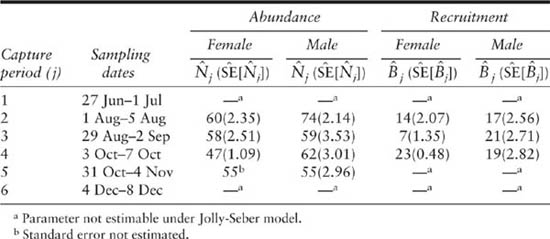
TABLE 5.4
Estimated seniority parameters (γ_j) and population growth rates (λ_j) under the temporal symmetry models (ϕ_t, p_t, γ_t) and (ϕ_t, p_t, λ_t) of Pradel (1996) for capture–recapture data on adult male and female meadow voles at Patuxent Wildlife Research Center

5.6 The Robust Design

The JS model has been widely used in animal population ecology, but it has long been known that estimates of survival probability are more robust to deviations from model assumptions than estimates of abundance (e.g., see Carothers 1973b; Gilbert 1973). As a means of dealing with this difference in robustness, Pollock (1981a, 1982) suggested sampling at two temporal scales, with periods of short-term sampling over which the population is assumed to be closed, and longer-term sampling over which gains and losses are expected to occur (Lefebvre et al. 1982). He recommended that the closed models of Otis et al. (1978) be used to estimate abundance with the data arising from each of the short-term sampling episodes. These data then can be pooled (with each animal recorded as caught if it was observed at least once during the closed population sampling) to estimate survival based on the CJS estimators. Recruitment can be estimated using the abundance estimates from the closed models and survival estimates from the open models (Pollock 1982).

The robust design consists of k primary sampling occasions, between which the population is likely to be open to gains and losses. At each primary sampling occasion j, a short-term study is conducted, with the population sampled over l_j secondary sampling periods during which it is assumed to be closed, although this assumption can be relaxed (Schwarz and Stobo 1997; Kendall and Bjorkland 2001). As an example, a small mammal population might be trapped for five consecutive days every two months, in which case, l_j = l = 5.

Capture–recapture data from the robust design can be summarized as number of animals exhibiting each capture history, where a capture history contains information about both secondary and primary periods. For example, a study with k = 4 primary sampling periods and l = 5 secondary sampling periods within each primary period would produce a capture history with 20 columns. A history for a particular animal might be

01101 00000 00100 10111

consisting of four groups of five capture values. The first group of five numbers gives the capture history over the five secondary periods of primary period 1, showing that the animal was captured on secondary occasions 2, 3, and 5 of primary period 1. The second group of numbers indicates that the animal was not captured at all during primary period 2. In primary period 3 it was captured on the third secondary occasion, and in primary period 4 it was captured on secondary occasions 1, 3, 4, and 5.

Under Pollock’s (1981a, 1982) original robust design, abundance was estimated with closed models using secondary capture history data, survival rates were estimated using standard open models with capture-history data reflecting captures in each primary period, and the number of new recruits was estimated using the closed-model abundance estimates and open-model survival estimates. Thus, the modeling proceeds via independent selection of an open model that incorporates survival and capture probabilities for the primary periods, and a closed model that incorporates abundances and capture probabilities for the secondary periods.

The likelihood-based approach to the robust design (Kendall et al. 1995, 1997) differs from the ad hoc approach in that a full likelihood is described for data from both secondary and primary periods. The full likelihoods are written as products of components corresponding to the two types of data, with mathematical relationships among the capture parameters of the components. Define the capture probability parameters

p_jg = probability that an animal is captured in secondary period g of primary period j; and

= probability that an animal is caught on at least 1 secondary period of primary period j.

These parameters, p_ig, , are related through the following expression:

Thus, an animal must be missed (not caught) in each of the secondary periods of primary period j to be missed in primary period j.

Consideration of the number of possible ways of modeling survival in the open-model framework and modeling capture probability in both the closed and open frameworks leads to the conclusion that the number of possible robust design models is large (Kendall et al. 1995). At one time, the inability to obtain maximum likelihood estimates for closed-population models that incorporated heterogeneous capture probabilities removed this class of closed models from consideration for joint likelihoods. However, the finite mixture models of Norris and Pollock (1996b) and Pledger (2000) now permit modeling of heterogeneity in a likelihood framework, so virtually any sort of closed model can be included in a joint likelihood. Reduced-parameter models, multiple-group models, multiple-age models, models with capture-history dependence, reverse-time models, time-specific and individual covariate models, and multistate models can all be used to develop joint likelihoods for robust design data (e.g., Kendall and Nichols 1995; Kendall et al. 1997; Nichols and Coffman 1999; Nichols et al. 2000; Lindberg et al. 2001; Kendall and Bjorkland 2001).

Assumptions underlying joint likelihood models for robust design data basically represent a union of the assumptions underlying the closed and open models that are combined. The important exception involves the capture probability parameters that are shared by the two components of the likelihoods. In the presence of temporary emigration, the relationship of equation 5.11 does not hold, as the complement of includes temporary emigration, whereas the complements of the p_jg reflect only the conditional probability of being captured, given presence in the sampled area (see below). In this situation, the models based on equation 5.11 will yield biased estimates, and appropriate models must incorporate the possibility of temporary emigration. Such models have been developed by Kendall and Nichols (1995), Kendall et al. (1997), Schwarz and Stobo (1997), and Kendall and Bjorkland (2001).

Temporary Emigration

Kendall et al. (1997) introduced random and Markovian models for temporary emigration, both of which are based on the concept of a superpopulation of animals. These animals are associated with the area sampled at period j, in the sense that they have some nonnegligible probability of being in the area exposed to sampling efforts during period j. Some number N_j of these animals are actually in the area and therefore are available for possible capture with probability . The models of Kendall et al. (1997) assume that the population is closed to gains and losses (including temporary emigration) over the secondary periods of primary period j, but this assumption can be relaxed if necessary (Schwarz and Stobo 1997; Kendall and Bjorkland 2001).

Define a new capture probability parameter associated with the super-population:

= the probability that a member of the superpopulation at primary period j (one of the animals in the superpopulation) is captured during primary period j.

The capture probability parameter under the robust design now corresponds to the probability that an animal exposed to sampling efforts at j (one of the N_j animals) is captured during j. This capture probability can thus be viewed as conditional on presence in the sampled area. The survival rate, ϕ_j, is redefined to reflect the probability that a member of the superpopulation at time j is still alive and a member of the superpopulation at time j + 1.

The model for random temporary emigration (Kendall et al. 1997; Burnham 1993) requires parameters η_j representing the probability that a member of the superpopulation at period j is not in the area exposed to sampling efforts during j (i.e., is a temporary emigrant). Thus, the expected number of animals in the area exposed to sampling efforts can be written as

It is also possible to specify the relationship between the capture probabilities for animals that are exposed to sampling efforts at j (), and for those in the entire superpopulation, regardless of whether or not they are exposed to sampling efforts at j (). This is

equation 5.12 simply specifies that for a member of the superpopulation to be caught at any period j, it must be in the area exposed to sampling efforts and then be captured.

The joint likelihood models that incorporate random temporary emigration model the secondary period data in the usual way with written as a function of capture probabilities for closed-population models. These closed-population models permit estimation of capture probability conditional on presence in the sampling area and exposure to sampling efforts. In the open-model portion of the likelihood, however, is substituted for the capture probability parameters, reflecting the possibility that the animal may not be in the area exposed to capture efforts. Such modeling permits direct estimation of conditional capture probability and temporary emigration probability η_j.

Kendall et al. (1997) also developed a class of more general models, in which the probability of being a temporary emigrant at primary period j depends on whether or not the animal was a temporary emigrant at time j – 1. Specifically, let denote the probability that a temporary emigrant at primary period j – 1 (i.e., was included in ) is also a temporary emigrant at time j. Let denote the probability that a nonemigrant at j – 1 is a temporary emigrant at j. Temporary emigration is thus modeled as a first-order Markov process.

To illustrate the Markovian model of temporary emigration, consider the probability associated with primary-period capture history 01010, which is

The above expression includes two possibilities, the probabilities for which are added together inside the first set of brackets. The first possibility is that the animal released at period 2 was a temporary emigrant at period 3. The second possibility is that the animal was not a temporary emigrant at period 3, but was simply not caught then. These two possibilities require two different temporary emigration parameters for period 4, reflecting the different emigration status at period 3.

Recruitment Components

Capture–recapture modeling for open populations provides estimates of gains to, and losses from, the sampled population. Sometimes it is of interest to decompose rates of gain into components associated with immigration and in situ reproduction. This separation is possible with the robust design using an approach described by Nichols and Pollock (1990); see also Pollock et al. (1990). Similarly, a reverse-time approach can be used to directly estimate the proportional contributions of immigration and in situ reproduction to population growth (Nichols et al. 2000).

Estimation

Robust design models with no temporary emigration and with both random and Markovian temporary emigration yield product-multinomial likelihoods. Similarly, multiple-age reverse-time modeling is based on a multinomial likelihood. Maximum likelihood estimation under most of these models is accomplished using programs MARK (White and Burnham 1999), RDSURVIV (Kendall and Hines 1999), and ORDSURVIV (Kendall and Bjorkland 2001).

5.7 Discussion

The number of capture–recapture models developed for open animal populations has increased greatly in the last two decades. This increase was made possible by high-speed computers that are able to maximize likelihood functions numerically. Between the mid-1960s and the mid-1980s, the only models available to biologists were those for which closed-form estimators had been derived (Cormack 1964; Jolly 1965; Seber 1965; Robson 1969; Pollock 1975, 1981b; Brownie and Robson 1983).

During the mid-1980s, open models requiring iterative computer solutions were developed with accompanying software (Cormack 1981; Sand-land and Kirkwood 1981; Jolly 1982; White 1983; Conroy and Williams 1984; Clobert et al. 1985; Crosbie and Manly 1985; Brownie et al. 1986; Burnham et al. 1987). For the last 15–20 years, flexible software such as SURVIV (White 1983), SURGE (Pradel et al. 1990), and now MARK (White and Burnham 1999) has permitted quantitative biologists to participate in the modeling process. This greater involvement of biologists in model development has led to a proliferation of models tailored to a variety of organisms and specific sampling situations.

The net result of this recent increase in development of open models has been an interesting shift of burden from the statistician to the field biologist. During the 1960s and 1970s, the rate of model development was limited by statisticians, as the burden fell to this group to develop the models and estimators needed to deal with various biological and sampling situations. However, over the last 15 years, statisticians and quantitative biologists have responded to this challenge and developed models and estimators for extremely complex biological and sampling scenarios. The burden has thus shifted to the biologist to conduct the appropriate experiments and collect the data needed to support these often-complicated and parameter-rich models of biological phenomena.

Finally, we note that an important future direction for capture–recapture modeling for open populations involves combination of capture–recapture data on sample areas with other data sources. Some joint models have been developed already (Freeman et al. 1992; Burnham 1993; Barker 1997, 1999; Powell et al. 2000, Besbeas et al. 2002, 2003) and others have been proposed (e.g., Bennetts et al. 2001; Nichols and Hines 2002). Such joint models offer the possibility of integrating seemingly disparate methods of studying and monitoring animal populations by bringing all relevant data to bear on specific inference problems.

5.8 Chapter Summary

• Two types of model are defined for open populations. Cormack-Jolly-Seber (CJS) models are conditional on the number of animals released on each sampling occasion, whereas Jolly-Seber (JS) models use information on the captures of unmarked animals and are therefore not conditional on the captured animals. The CJS models allow for the estimation of capture and survival probabilities, while the JS models also allow the estimation of abundance and other related parameters.

• The probabilistic basis for CJS models is explained, and the assumptions are noted. Reduced-parameter versions of the models are reviewed, with capture or survival probabilities assumed to be constant over time. The models can be extended through the use of covariates to account for variation in parameters over time, variation in parameters among groups of individuals (e.g., males and females), and variation in parameters associated with individuals.

• Model selection and testing for goodness-of-fit are discussed.

• An example involving the trapping of meadow voles is used to illustrate the various methods.

• Models that allow parameters to vary with the known age of animals are discussed, including models for animals first released at age zero, and age-specific breeding models.

• Reverse-time models are reviewed as a means of estimating parameters associated with the recruitment process.

• The unconditional JS types of models are reviewed, including the use of Horvitz-Thompson estimators of population size, the super-population model of Crosbie and Manly, and the temporal symmetry approach for the estimation of a population growth rate. Methods are illustrated using the meadow voles example.

• The robust capture–recapture sampling design is described, involving several periods of intensive sampling when the population size can be assumed to be constant, separated by longer periods during which the population size is expected to change. Estimation methods specific to this design are reviewed, including the allowance for temporary emigration.

• The general development of models for open-population capture–recapture data in the past is discussed, and likely future developments are anticipated.

Figure 5.3. Visible implant alpha-numeric tag in steelhead (Oncorhynchus mykiss) smolt. (Courtesy of Northwest Marine Technology, Inc.)