Seven

Joint Modeling of Tag-recovery
and Live-resighting Data

RICHARD J. BARKER

7.1 Introduction

Between 1985 and 1990, 6160 paradise shelducks (Tadorna variegata) were banded in a study carried out in the Wanganui Region, New Zealand. Molting shelducks were trapped in January and birds checked for tags. Marked birds had their number recorded and were then released; unmarked birds were marked and released. Between marking occasions birds were also reported shot by hunters, so the reencounter data represents a mix of live recaptures, for which the models of chapters 3 and 5 are suitable, and dead-recovery data, for which the models of chapter 6 are suitable. Because birds were reencountered in two ways, a fully efficient analysis requires new models that simultaneously model these two reencounter processes.

The Cormack-Jolly-Seber (CJS) model (chapter 3) and tag-return models (chapter 6) have dominated the analysis of mark–recapture data from open populations. In the CJS model the data are from a sequence of samples (referred to as the capture occasions) consisting of marked and unmarked animals, where captures and recaptures are obtained over a short period of time during which the population is assumed closed. These capture occasions punctuate longer periods during which the population is subject to births and deaths. In the tag-return models, by contrast, the capture occasions serve only to provide a succession of releases of marked animals and it is the returns from dead animals between release occasions that are modeled. The use of information from encounters of marked animals during the open interval between capture occasions is a key difference between the tag-return models and the live-recovery models.

As in the paradise shelduck study, animals marked and released during early sample occasions are often recaptured during subsequent sample occasions. Live recaptures in band recovery studies have traditionally been ignored, partly because of the technical difficulties in simultaneously modeling the two types of data, and because live recaptures during trapping have been uncommon. Nevertheless, in some studies, live recaptures may be substantial, particularly for nonmigratory species. Similarly, during a study based on live recaptures of marked animals information may also be available from recoveries of dead animals. Supplementing the live-recapture information with recovery data should lead to improved estimation.

Figure 7.1. Tusk-banded Pacific walrus (Odobenus rosmarus), Round Island, Alaska, 1982. (Photo by Steven C. Amstrup)

In a study where several kinds of information are available, ignoring one of the sources so that a simple model, such as CJS or tag-return model, can be used means that parameter estimates will be less precise than they otherwise could be (Barker and Kavalieris 2001). A joint model contains extra parameters that are needed to model the data. When these extra parameters have a biological relevance, and when data are sufficient to allow meaningful estimation and interpretation, their inclusion will mean that the study is more informative. In short, use of a joint model may provide better parameter estimates and more informative biological interpretations without the need for more animals to be marked.

Animal Movement

Although both the CJS and tag-recovery models have parameters for survival, it has long been recognized that the two survival probabilities are fundamentally different. The difference between these probabilities derives from their treatment of emigration.

In mark-recapture studies it is often difficult to obtain a random sample of animals from the study population. More commonly, a local population is sampled and marked. In the paradise shelduck study a bird was only at risk of live recapture if it chose to molt at one of the locations where birds were captured and banded. Once banded, a bird could appear in a later live-recapture sample only if (1) it survived and remained in the local population being sampled, or (2) it survived, left the local population, and then returned. Jolly (1965) and Seber (1965) recognized this and insisted that any emigration be permanent. That is, animals may leave the study area but they may not return. The consequence is that the Jolly-Seber survival parameter, usually denoted ϕ_j, represents the joint probability that the animal remains at risk of capture and does not die between samples j and j + 1. In contrast, in tag-return models it is usually assumed that animals are exposed to the tag-recovery process (i.e., death and reporting) throughout their range. That is, there is no emigration from the study population. In this case there is no site fidelity component to the survival probability.

The assumption of permanent emigration in mark-recapture models is one that has been given relatively little attention. However, assumptions about movement should be based on known biology rather than mathematical convenience. For example, it may be unreasonable to insist that an animal that has moved off the study area cannot later return. In these studies it is important that the permanent emigration assumption be relaxed.

Burnham (1993) introduced random emigration as an alternative to the permanent emigration assumption. Under random emigration a marked animal may leave and reenter the study population, but the probability that it is at risk of capture at occasion j is the same for all animals. A generalization is Markovian temporary emigration where the probability an animal is at risk of capture at occasion j depends on whether or not it was at risk of capture at occasion j – 1 (Kendall et al. 1997). Permanent emigration represents an extreme case of Markov emigration in which the probability that an animal is at risk of capture at occasion j is zero for an animal not at risk capture at occasion j – 1.

7.2 Data Structure

To represent the different types of information in this study it is necessary to generalize the encounter history introduced in section 1.3. The format of program MARK (White and Burnham 1999; White et al. 2001) can be used to represent data from a study where animals can be reencountered by a live recapture, a live resighting, or a dead recovery. These events are summarized using a pair of indicator variables (L_j, D_j), with one pair for each of the j sampling periods. If at capture occasion j the animal is recaptured then L_j is assigned the value 1. Otherwise, it is assigned the value 0. If between capture occasion j and capture occasion j + 1 the animal is found dead and the tag is reported, then D_j is assigned the value 1. If instead the animal is resighted alive between capture occasions j and j + 1, then D_j is assigned the value 2. If the animal is not resighted or not recovered dead, between capture occasions j and j + 1, then D_j is assigned the value 0. Sometimes, an animal will be resighted alive and then be reported dead, with both events occurring in the interval j, j + 1. In such cases the indicator variable D_j is assigned the value 1, indicating that the animal was found dead and the earlier resighting is ignored.

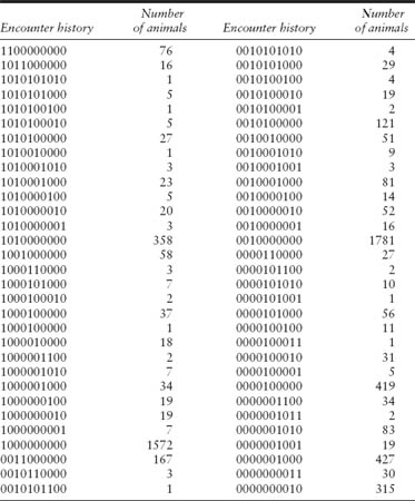
The encounter histories for the paradise shelduck study are given in table 7.1. For example, the 76 animals with the encounter history 1100000000 were marked and released in January 1986 and then reported dead during the 1986 hunting season, which took place between May and August. The 16 animals with the history 1011000000 were marked and released in January 1986, recaptured in January 1987, and then reported dead during the 1987 hunting season.

The parameters of the joint live-recapture and dead-recovery model are S_j, the true survival probability between sample occasions j and j + 1; F_j, the probability that an animal in the local study population does not leave the study population between samples j and j + 1; , the probability that an animal not in the local study population at the time of sample j is in the local study population at the time of sample j + 1; r_j, the probability that an animal that dies between samples j and j + 1 is found and its band is reported and p_j, which, as with capture–recapture models, is the probability of capture at occasion j.

7.3 Simple Models

Anderson and Sterling (1974) carried out an analysis of banding data from pintail ducks (Anas acuta) by modeling the live-recapture data separately from the tag-return data. Under the assumption that emigration is permanent, the Jolly-Seber survival estimator provides an estimate of F_jS_j. Here, S_j is the probability an animal alive at sampling occasion j is still alive at sampling occasion j + 1, and F_j is the probability that an animal at risk of capture at j is still at risk of capture at j + 1 (i.e., it has not permanently emigrated). The tag-return model provides an estimate of S_j, and Anderson and Sterling (1974) used the ratio to estimate the probability that ducks banded in year j were still at risk of capture in year j + 1.

TABLE 7.1
Encounter histories in program MARK format for the joint analysis of live-recapture and dead-recovery data from a study of paradise shelduck banded in the Wanganui Region, New Zealand between 1986 and 1990

Mardekian and McDonald (1981) proposed a method for analyzing joint band-recovery and live-recapture data that exploited the modeling approach and computer programs of Brownie et al. (1978, 1985).

Following release at a specific capture time, an animal may fall into one of three mutually exclusive categories:

1. the animal is found dead or killed and its band is reported (terminal recovery);

2. the animal returns to the banding site in a subsequent year and is captured; and

3. the animal is never seen again and its band is never reported.

 

Because animals can be recaptured several times, the full model allowing for all such recapture–recovery paths is difficult to write out. Mardekian and McDonald (1981) avoided this complication by ignoring intermediate recapture data and modeling the last encounter of each animal. The last encounter of each animal is either recovery of the band or the last live recapture. Mardekian and McDonald (1981) showed that from the tag-return model fitted to the last encounter is an estimate of the survival probability between i and i + 1.

The advantage of the Mardekian-McDonald analysis is the simplicity with which it can be carried out. The estimates can be obtained in a straightforward manner utilizing the procedures and software of Brownie et al. (1985). However, because intermediate live-recaptures are ignored, the Mardekian-McDonald survival rate estimator is not fully efficient. Another drawback of the Mardekian-McDonald analysis is that it is correct only if it is assumed that there is random or no emigration of animals. Under permanent or Markovian emigration it can be shown to lead to biased estimators (Barker 1995). When emigration is permanent, the estimator of Anderson and Sterling (1974) can be used instead, but it will also lead to biased estimates under Markovian emigration. Burnham (1993) established the foundation for an efficient analysis of the joint live-recapture and tag-return model. The basic model developed by Burnham (1993) combines the CJS model with the time-specific band-recovery model M1 of Brownie et al. (1985). That is, recapture, recovery, survival, and movement probabilities are time-specific and there is no heterogeneity. Burnham’s (1993) model offered the alternative movement assumptions of random or permanent emigration.

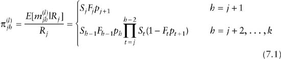
As in the CJS model, the likelihood function for the joint model is proportional to the joint probability of the observed recapture and recovery events for the animal. It is known that the 76 animals with the encounter history 1100000000 in the paradise shelduck study died between January 1986 and January 1987, and given that they died, their bands were found and reported. Therefore, the joint probability Pr(1100000000 | first release in 1986) = (1 − S₁)r₁. Similarly, it is known that the 16 animals with the history 1011000000 survived between 1986 and 1987, remained within the local population that was at risk of capture in January 1987 and were caught, and then they died between 1987 and 1988 and were reported dead. The joint probability of these events is given by

Under both random and permanent movement assumptions, joint live-recapture and dead-recovery data can be summarized using combined recapture and recovery array known as an extended m-array (table 7.2). An advantage of this summary using sufficient statistics is that it provides a basis for efficient goodness-of-fit tests for these models. The extended m-array is a simple generalization of a band-recovery array for model M₁ of Brownie et al. (1985). From the encounter histories, the extended m-array can be constructed by considering the first reencounter of an animal after release following a live recapture. In a study with k capture occasions, and where recoveries are obtained up until occasion g (g ≥ k), each of the R_j marked animals released at capture occasion j can next be encountered either by a live recapture in one of the samples at time j + 1, …, k or by dead recovery in one of the intervals between the capture occasions at times j, j + 1, …, g. If the number of animals released at time j and next encountered by live recapture at time h is represented by , and the number of animals released at time j and next encountered by dead recovery at time h by , then the data can be represented as in table 7.2. In this summary, the animals with the encounter history 1100000000 contribute to just . The animals with the history 1011000000 first contribute to through the live recapture at time 2.

TABLE 7.2
Extended m-array illustrating the combined recapture and recovery data necessary for a joint analysis of live-recapture and tag-recovery data Because they were released at time 2 they are included in the R₂ animals released at time 2, and then they contribute to . The extended m-array for the Wanganui paradise shelduck study is given in table 7.3.

TABLE 7.3
Extended m-array illustrating the joint live-recapture and tag-recovery data from the paradise shelduck (Tadorna variegata) banding study in the Wanganui Region, New Zealand, 1986–1990

Under the assumption that the fates of each animal in a release cohort are independent, the data in the extended m-array can be modeled using multinomial distributions. Each release cohort represents an independent multinomial experiment. Under random emigration, the probabilities associated with the statistics in Table 7.2 are given by

and

To see that this provides the correct probability structure under random emigration, consider an animal released at occasion j and next captured at time j + 2. It is known that it survived from occasions j to j + 1 and from occasions j + 1 to j + 2, and that it was caught at occasion j + 2. What is unknown is whether it was at risk of capture at time j + 1. However, there are just two mutually exclusive possibilities. The first possibility is that the animal was at risk of capture at time j + 1, but not caught, which occurs with probability F_j(1 – p_{j + 1}). The animal then remained at risk of capture and was caught at time j + 2, which has probability F_{j + 1}P_{j + 2}. The second possibility is that the animal temporarily emigrated between time j and j + 1, which occurs with probability (1 – P_j), and then it returned to the local study population and was caught, which has probability F_{j + 1} p_{j + 2}. The probability that it was next captured at j + 2 given that it was released at j is therefore

which reduces to

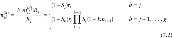
Under permanent emigration the situation is complicated by the fact that although animals can permanently emigrate from the local study population and no longer be at risk of capture, they are exposed to dead recovery throughout their range. Under permanent emigration the multinomial cell probabilities are given by

and

where

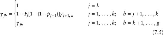
and is the probability that an animal alive and at risk of capture at capture occasion j, and alive at h, is not captured between occasions j and h. Computation of the γ_jh parameters is done recursively for any h by iterating backward from j = h, h − 1, . . . , 1 (Burnham 1993).

Because the multinomial cell probabilities differ between the two forms of emigration in the joint model they do not have the same likelihood and the two types of emigration, random or permanent, can be distinguished. However, under random emigration the parameters F_j and p_{j + 1} (j = 1, . . . , k − 1) are confounded as they always appear in the model as the product F_j p_{j + 1}. Under permanent emigration, the joint model allows estimation of F₁, . . . , F_{k − 2} but the pair F_{k − 1} and p_k are confounded.

Parameter Estimation

Under permanent emigration, closed-form maximum likelihood estimators (MLEs) and their variances do not exist for Burnham’s (1993) joint model except in very restrictive cases. Instead, numerical solutions to the likelihood function must be found using a suitable software package. Under random emigration closed-form MLEs do exist and in terms of the notation in table 1.1 are given by

and

where

and z_j is the number of marked animals in the population at occasion j that were not caught at j, so that z₁ = 0 and . The dot in place of an index indicates summation across the replaced index. For example, , and is the number of the R_j animals in the jth release cohort that were ever encountered again. Similarly, is the total number of live recaptures in the jth interval and is the total number of dead recoveries between j and j + 1. These summary statistics are all easily obtained from the modified m-array (table 7.3). The z_j also can be obtained from the m-array as the sum of the values in the upper submatrices (for capture and dead recovery) above the occasion in question. Hence, the z₁₉₈₇ = 214 is derived from the numbers shown in bold in table 7.3.

These summary statistics are presented more compactly in table 7.4, where we find (the number of marked animals immediately before the first sampling occasion is always zero) and , which gives

A full set of estimates computed from the data in table 7.4 is given in table 7.5.

Estimators for the sampling variances are

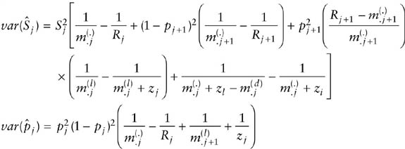
and

TABLE 7.4
Summary statistics for the joint live-recapture and tag-recovery data for paradise shelduck (Tadorna variegata) banded in the Wanganui Region, New Zealand, 1986–1990, where R_j is the number of marked animals released at occasion j.

where

It is useful to note that is the same as under the CJS model but with the statistics R_j, , and z_j augmented by the dead recoveries, and with the addition of the term . Because of this extra term, simply plugging the augmented statistics into the CJS variance estimator will underestimate the true sampling variance. The extra term can be thought of as a penalty term that adjusts the variance estimator to account for the estimation of the reporting parameter r_j.

TABLE 7.5
Parameter estimates for the joint live-recapture and tag-recovery data for paradise shelduck (Tadorna variegata) banded in the Wanganui Region, New Zealand, 1986–1990 under random emigration

Assumptions

Key assumptions of the above model are that fates of animals are independent and that parameters differ only by time and not among individual animals or according to the capture history. In addition, it is important that the recapture process operates over a short period of time during which the population can be considered closed. Note that the population does not need to be closed during the dead-recovery interval, which may be the entire time between live-capture occasions. If specific effects are believed present that mean the assumptions do not hold, the model may be modified accordingly. There have been a number of developments extending the above models to account for specific structure in the analysis. Some of these are introduced in the next section. It is also desirable to have a method for assessing how well a particular model accounts for variation in the data.

Goodness-of-fit tests comprising two sets of contingency tables similar to TEST2 and TEST3 of Burnham et al. (1987) can be constructed for these models. The theoretical basis of these tests is given by Barker (1997) for the joint models and extends the work of Pollock et al. (1985) and Brownie and Robson (1983) for live-recapture and tag-resighting studies and by Brownie et al. (1985) for tag-recovery models.

The first set tests whether the next encounter following the current live capture depends on the previous capture history and generalizes TEST3 of program RELEASE (Burnham et al. 1987). The test is valid under random, permanent, or Markov emigration. For the 1988 release cohort in the paradise shelduck study, the full contingency table for the first test component is given in table 7.6. This table is found by classifying each of the animals that were released in 1988 first according to their capture history before the 1988 release (i.e., identification of subcohorts), and second according to when and how they were next encountered. Although the recapture and recovery patterns for each subcohort appear similar in table 7.6, more of the newly marked birds were never seen again (433/577 = 0.75) than the birds that had been caught at least once before

(chi-square statistic = 8.17 with 4 df, p = 0.004). There are several reasons why this could happen, including temporary trap shyness resulting from first capture, an age effect (since newly marked cohorts tend to include younger birds), or the presence of transients (Pradel et al. 1997a) in the population.

TABLE 7.6
Contingency table for the 1988 release cohort testing whether the classification of birds according to when they were next encountered depends on their capture history prior to release in 1988

Under random emigration, a second set of goodness-of-fit tests can be constructed that generalize TEST2 of RELEASE (Burnham et al. 1987). These are found by partitioning the animals known to be alive immediately following capture occasion j first according to whether or not the animals were captured at time j + 1 and second according to how and when the animals were next encountered after time j + 1.

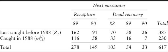
The full contingency table for this test component constructed from marked paradise shelduck known to be alive immediately after the 1988 sample is given in table 7.7. The counts in the contingency table suggest that birds not caught in 1988 have recapture and recovery patterns similar to those of birds caught in 1988, although there is weak evidence against the model (chi-squared statistic = 8.73 with 4 df, p = 0.07). Possible reasons for this test indicating lack of fit include a temporary effect of capture on the pattern of recapture or dead recovery and failure of the random emigration assumption.

TABLE 7.7
Contingency table for the marked birds known to be alive immediately after the 1988 sampling occasion testing whether recapture or recovery after the 1988 sample depends on whether or not the bird was caught in the 1988 sample

An overall test statistic is obtained by pooling results from all the contingency tables constructed as above. For the paradise shelduck study there are seven contingency tables in all, and summing across these yields a chi-squared statistic of 56.95 with 16 df (p < 0.0001), providing strong evidence that the model is not adequate.

If emigration is permanent or Markovian, the second set of goodness of fit tests generalizing TEST2 described above are not valid. Instead, a test can be constructed by comparing the observed and expected values of the m-array. Each row of the m-array corresponds to a particular release cohort and yields a test-statistic. An overall test statistic is obtained by summing across each row of the m-array. Although the same procedure can be followed for random emigration, the contingency table test described above will be more efficient.

7.4 More General Models

If key model assumptions are violated then biased estimation will likely result. In addition, sampling variance estimates may be biased. Structural inadequacy of the model may be apparent from goodness-of-fit testing, or there may be theoretical reasons for believing that the model is inadequate. The joint model of Burnham (1993) has been generalized in two key ways.

Catchpole et al. (1998) relaxed the assumptions to allow both age- and time-dependent parameters. A more general extension of the model is included in the computer program MARK (White and Burnham 1999; White et al. 2001). In addition to age and time dependence, MARK allows the parameters in the model to depend on individual covariates and also allows environmental covariates that can be used to explain time variation in the parameters.

The joint live-recapture, live-resighting, and tag-recovery model of Barker (1997) and Barker et al. (2004) covers the general situation where there are live recaptures, live resightings from any time between the capture occasions, and dead recoveries that occur any time between marking occasions. The joint live-recapture, live-resighting, and tag-recovery model provides three important generalizations of tag-resighting and tag-return models. First, it allows information from recaptures of marked animals during the tagging occasions to be included in the analysis. Second, it relaxes the assumption that the population is closed during the resighting period. Third, it allows Markovian temporary emigration as well as the special cases of permanent and random emigration.

In addition to the parameters of Burnham’s joint model, Barker’s model introduces two more resighting parameters. The first is ρ_j, which is the probability a marked animal alive at sampling occasions j and j + 1 is resighted between j and j + 1. The second is , which is the probability that an animal that dies between occasions j and j + 1, but that was not found and reported, was resighted alive between j and j + 1 before it died.

The CJS model, the tag-recovery model, and Burnham’s joint live-recapture dead-recovery model are special cases that arise by making appropriate constraints on the parameters. For example, constraining the live resighting parameters ρ_i and to equal zero leads to Burnham’s (1993) joint model but with Markovian emigration. Another special case arises by assuming no live recaptures but resighting over an open period between the capture occasions in which newly marked animals are released. The survival parameters in this model can be estimated and it represents a model that can be validly applied in a tag-resighting study with an open resighting interval.

7.5 Model Fitting and Assessment

As for Burnham’s joint model, closed-form maximum likelihood estimators exist only under the random emigration assumption and are given by Barker (1997). Under permanent or Markov emigration numerical methods must be used to find solutions to the likelihood equations. The model can be fitted using the likelihood constructed directly from the encounter histories (Burnham 1993).

The likelihood function is constructed in a similar manner to that for Burnham’s (1993) joint model. Consider a bird in the paradise shelduck study that was released in 1986, resighted alive between 1986 and 1987, that was captured in 1987, then reported shot during the 1987 hunting season. This bird would have the encounter history 1211000000 with the associated probability

Because we know that this animal was alive in 1987, the resighting event is coded with the parameter ρ₁, the probability an animal alive at times 1 and 2 is resighted alive in this interval. The parameter , the probability that an animal that dies between times j and j + 1 without being reported dead is resighted before it dies, enters into the likelihood function only for animals that are never seen again following a live resighting. For example, consider a bird released in 1990, the last capture occasion, that was resighted alive between 1990 and 1991. It is not known whether this bird was alive in January 1991; therefore, the probability of the encounter history is given by

Direct modeling of the encounter histories is very flexible, because parameters can be modeled using explicit functions of covariates that may vary over time, or by individuals, using a generalized linear model formulation. If θ_ij is a parameter unique to individual i at time j, then covariates can be included in the model by using the expression η_ij = β₀ + β₁ x_j + β₂x_j where η_ij = h (θ_ij) is the link function (McCullagh and Nelder 1989), β₁ is a vector of effects for time-specific covariates x_j, and β₂ is a vector of effects for individual-specific covariates x_j. The generalized linear model formulation offers much flexibility. For example, with a little thought joint models that allow age-dependence and short-term marking effect can be fitted.

To introduce a short-term marking effect on survival using individual covariates, survival is modeled as h(S_ij) = β_0j + β_1jx_ij, where x_ij = 1 if animal i is marked and released for the first time at time j, or 0 otherwise. This approach allows the models of Pollock (1975) and Brownie and Robson (1983) to be extended to incorporate live recaptures and tag recoveries, and the models of Brownie et al. (1985) to be extended to include live recaptures. Barker (1999) developed explicit estimators and tests for age dependence and short-term marking effect but only under the random emigration assumption.

A very large number of models can be fitted to a data set by including those models that are constructed by placing restrictions on parameters. In a study where animals are classified according to sex, parameters can be constant, sex-specific, time-specific, or sex- and time-specific. With seven parameter types in the model for the joint analysis of live-recapture, live-resighting, and dead-recovery data, 16,384 models can be constructed by considering all combinations of this nature. Because the resighting parameters ρ_j and model similar events, as do the movement parameters F_j and it may be reasonable to consider just models where the same effects apply to each member of the pair. Even so, there are still 1024 models that can be constructed in this case.

The very large number of potential models compared to the CJS or tag-return models means that more realistic models can be constructed, but it also emphasizes the need for sensible model-selection strategies and efficient model-selection algorithms, such as those based on Akaike’s Information Criterion (chapter 1). Because it is not practical to fit all possible models it is important to think about the effects that are likely to be present before fitting models. For example, in most studies researchers have little or no control over the tag-recovery and resighting processes. In this case time-varying reporting and resighting parameters will probably be needed in the model. In species that are not sexually dimorphic and where males and females behave similarly there may not be a sex effect on reporting or resighting parameters.

A related issue is that joint models have many more parameters than their live-recapture or tag-recovery counterpart. In the paradise shelduck example described below where there are just five capture occasions and no separation of birds by sex, the fully time-dependent model with no individual covariates has 31 parameters. The equivalent CJS model with six sampling periods has just eight parameters. It might be thought that the need to estimate extra parameters will reduce the precision of the survival rate estimates. However, as shown by Barker and Kavalieris (2001), this is not the case. The CJS and tag-recovery models are special cases of the joint models, and the survival probability can be estimated under both models without the extra information provided by the joint model. The extra parameters are required only to model the additional data. If there is little useful information in the additional data, the extra parameters will be poorly estimated, but not the survival rates.

Goodness-of-Fit

The tests described above for the analysis of live-recapture and dead-recovery data were developed by Barker (1997) for the more general situation where there are live resightings as well. Accordingly, the two components described above differ slightly in the more general case. Importantly, the m-array represents a set of sufficient statistics only under random emigration for this more general model so the tests described here are valid only in the case of random emigration. As in the tests above, the first set of tests is used to assess whether the next encounter following the current live encounter depends on the encounter history to date. Including live resightings means there are now a greater number of histories possible before and after the current encounter.

The second set of tests partitions the animals known to be alive immediately following capture occasion j according to whether they were (1) caught at j, (2) resighted alive between occasions j − 1 and j, but not caught at j, and (3) not resighted between j − 1 and j, and not caught at j. Because Burnham’s (1993) model does not include live resightings, this partitioning reduces to whether or not the animals were recaptured at time j + 1 in his model. The second partition is according to how and when the animals were next encountered after time j + 1. This test examines whether an encounter between occasions j and j + 1 has longer-term effects on the probability of later encounters, and generalizes TEST2 of RELEASE (Burnham et al. 1987).

In addition to the two components described above a third set of contingency tables are based on two partitions of the marked animals that are known to be alive at sample time j − 1 and just before sample j. The first partition is according to whether or not they were captured at j. The second is according to whether they were resighted alive between occasions j − 1 and j. The cross-classification arising from the two partitions generates contingency tables that test whether resighting has a short-term effect on the probability of recapture. This test is not relevant for Burnham’s (1993) model because the model does not involve live resightings.

The usefulness of these tests is questionable because they test the fit of the joint models only under random emigration and not in the more general case of Markov emigration. However, the comparison of expected and observed values in the contingency tables may still be useful for highlighting model inadequacies. If emigration is not random, a goodness-of-fit test can be constructed using a parametric bootstrap procedure provided there are no individual covariates. In the parametric bootstrapping procedure data are simulated under the assumed model using the parameter estimates for the parameter values. The simulation process is repeated a large number of times, and each time the value of the deviance statistic (equation 1.4 with L₂ computed for a saturated model) is recorded. If few of the simulated deviance values exceed the value for the observed data, this is taken as evidence that the data are inconsistent with the assumed model.

A philosophical objection to a goodness-of-fit test is that there is never complete faith in assumptions. The model is just an approximation to reality, and will fail the test given enough data. An alternative approach is to have a measure of the extent to which the model fails to represent the data. The overall goodness-of-fit statistic for the whole model, however it is calculated, divided by its degrees of freedom is one such estimate of the extent of lack of fit. This is the statistic of equation 1.8.

Two important types of failure of the model are when, first, the fate of one animal influences the fate of another, and, second, when parameters are not the same for each animal. If fates are not independent, or if parameters vary randomly from animal to animal, the data will often be overdispersed relative to the model. If the data are overdispersed, the parameter estimators are unbiased but model-based standard errors will be too small. Quasi-likelihood (section 1.4) has been suggested as a method for approximating the true sampling model for the data, where the variances of the parameters are the same as for the model with no overdispersion except that they are multiplied by the estimated scaling constant .

With mark–recapture models can be found in one of two ways. The first is to use an explicit goodness-of-fit test, as outlined above, to find an overall χ² statistic and its associated degrees of freedom, d. The estimator then provides an estimate of c. The second approach is to use the parametric bootstrap method. The approach recommended by White et al. (2001) is to divide the observed deviance for the data by the mean of the simulated deviances. The mean of the simulated deviances represents the expected value of the deviance under the null hypothesis that the model is correct. Therefore, the observed deviance divided by the expected deviance is an estimate of the overdispersion in the data. With overdispersion, the variances of the parameter estimates are underestimated by a factor of 1/c. Therefore, the estimate can be used to scale up the sampling variances to correct for overdispersion.

7.6 Tag Misreads and Tag Loss

Because the joint models incorporate information provided by members of the public, data quality is an important issue. Misreading of tag numbers may be more common than in studies in which a limited number of project personnel perform the work. Similarly, misreading of tags is likely to be more of a problem in resighting studies than in studies where animals are captured, because errors in reading tags are more likely when tags are read at a distance. The effect of misread tags in a CJS-type study has been investigated by Schwarz and Stobo (1999). They showed that estimates of survival rate can be biased early on in the study, but that this bias tends to ameliorate later in the study. Schwarz and Stobo (1999) also developed a model for tag misreading that allows misread rates to be estimated using CJS data. Effects of tag loss can be similar to those of tag misreads. Large, high-visibility tags used in a resighting study may be prone to tag loss. Double tagging may help assess rates of tag loss (Fabrizio et al. 1999), but loss of tags from double-tagged animals may not be independent. This confounds efforts to assess loss rates (Bradshaw et al. 2000; Diefenbach and Alt 1998). The Schwarz and Stobo (1999) misread model also may be extended to studies involving double tagging. Pollock (1981), Chao (1988), Nichols et al. (1992a), and Fabrizio et al. (1999) have suggested a variety of methods to assess tag loss and how to mitigate its effects on estimation of population parameters.

7.7 Computing Considerations

Currently, the only widely available computer packages that allow the user to fit joint models efficiently are the packages SURVIV (White 1983) and MARK (White and Burnham 1999). SURVIV is useful in those cases where the model can be fitted to the extended m-array. Unfortunately, for the models discussed in this chapter, this restricts the use of SURVIV to the joint live-recapture, dead-recovery models based on Burnham’s (1993) model, or the joint live-recapture, live-resighting, and dead-recovery model based on Barker’s (1997) model under the assumption of random emigration.

One advantage of SURVIV is that it automatically includes a goodness-of-fit test. This test, however, is not fully efficient for the models considered in this chapter because it does not include the first component of the tests described above, that component can be thought of as assessing the sufficiency of the m-array. Disadvantages of SURVIV are, first, that the user needs to code the algebraic structure of the model by hand before the model can be fitted. Equations 7.1 to 7.5 in Burnham (1993) can help with this. Second, SURVIV is not suitable if the user wishes to include individual covariates in the analysis.

Program MARK (White and Burnham 1999) fits the joint models described above using a likelihood function constructed directly from the encounter histories. A generalized linear model formulation is used to introduce individual covariates into the model. This process is very flexible as parameters can be indexed by release cohort, time, or individual. Because not all parameters can be estimated in a completely cohort- and time-specific model, constraints are introduced through a parameter index matrix (PIM). Model assessment in MARK for joint live-recapture, live-resighting, and dead-recovery models is carried out using parametric bootstrapping.

By fixing parameters it is possible to fit restricted versions of the joint model. For example, by constraining the resighting parameters ρ_j and to equal zero, the joint model for live recaptures, live resightings, and tag recoveries can be used to fit Burnham’s joint model. This is currently the only way to fit a Markovian emigration model in MARK to joint live-recapture and tag-recovery data. If the capture probabilities p_j and the tag-reporting probability r_j are constrained to equal zero, it is possible to fit a tag-resighting model that allows the population to be open during the resighting period.

The permanent emigration model can be fitted using MARK by setting all the equal to zero. Under random emigration, = F_j, but F_j is now confounded with the capture probability p_{j + 1}. A useful computational trick is to set the constraint F_j = 1. Because F_j and p_{j + 1} always appear in the product F_j p_{j + 1}, this ensures that the numerical procedure will find estimates of p_{j + 1} that correspond to F_j p_{j + 1}. Under the constraint F_j = 1, the parameters F_j will make no contribution to the likelihood and so can be arbitrarily constrained to any real value.

In many studies data will be too sparse to allow all parameters to be estimated. MARK will successfully maximize the likelihood in this situation, but the estimates of the inestimable parameters will not be unique, which is usually indicated by a very large estimated standard error. MARK attempts to determine which parameters are uniquely estimated using numerical methods, and usually does so correctly if the default sin link is used. For other link functions, the parameter count may not be correct and this usually happens when some of the parameter estimates are at their boundary value, for example, a survival rate estimated to be 1.0.

TABLE 7.8
Model fitting summary from fitting the fully time-dependent Markov, permanent, and random emigration models to the paradise shelduck data

TABLE 7.9
Parameter estimates for the paradise shelduck data under random emigration from program MARK

Different models can be compared in MARK using the small-sample version of Akaike’s Information Criterion (AIC_c) mentioned in chapter 1 for model selection. As an illustration, table 7.8 gives model fitting information for the three different movement models fitted to the paradise shelduck data. AIC_c indicates a preference for the permanent emigration model (Akaike weight = 0.608) or possibly the Markov emigration model (Akaike weight = 0.372) with much less support for the random emigration model. An estimate of the overdispersion scaling parameter c for the Markov emigration model, the most general of the three models, indicates considerable overdispersion . Also, of 1000 simulated deviance statistics, all were less than the deviance statistic for the data of 120.458. This suggests that there may be some structural inadequacies in the model for the paradise shelduck data. For comparison with the explicit solutions, the parameter estimates given by MARK for the random emigration model are given in table 7.9.

7.8 Chapter Summary

• An Example involving the banding of paradise shelducks is used to introduce situations where some marked animals are recovered alive and others are recovered dead. It is noted that it will be more efficient to produce parameter estimates from both types of recovery, rather than considering the information from either live or dead recoveries only.

• The effect of animal movement on the standard models for live and dead recoveries is discussed.

• The structure of the data from a study involving both live and dead recoveries is described.

• Simple early models that use both live- and dead-recovery data are discussed, including the Burnham model, which makes use of all of the available data and assumes that recapture, recovery, survival, and movement probabilities vary with time. The assumptions needed for estimation and goodness-of-fit tests are reviewed.

• A generalization of the Burnham model that allows parameters to vary both with age and time is discussed, as is another generalization that allows for temporary migration. Model fitting and assessment methods are discussed for the second of these models.

• The effects of misreading of tags and tag loss are discussed.

• Methods for computing estimates using data on live and dead recoveries are described.

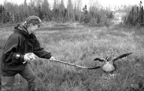
Figure 7.2. Martha Tomeo creatively avoids being attacked by a neck-collared Canada goose (Branta canadensis), as she checks a nest near Anchorage, Alaska, 2000. (Photo by Jerry Hupp)