
Six
Tag-recovery Models
6.1 Introduction
Modern tagging models for estimating mortality rates of exploited populations derive from the work of Seber (1970), Brownie (1973), Youngs and Robson (1975), and Brownie et al. (1985). These models pertain to the case where tagged animals are killed when they are recaptured and there is no direct information on animals that die of natural causes (such as empty shells of mollusks). The authors cited above concentrated on the estimation of the annual survival rate, S, which is the probability that an animal alive at the start of the year will survive to the end of the year. These models commonly are called Brownie models. Rates of harvesting can also be derived from Brownie models under special circumstances. However, a class of models known as instantaneous rates models has also been developed specifically for estimating fishing or hunting mortality and natural mortality (the latter being the rate of mortality due to all causes other than harvesting).
Modern tagging models are based on the following logic. If two tagged cohorts of animals that are completely vulnerable to hunting or fishing are released exactly one year apart in time, then the fraction of the tags recovered in a unit of time (any time after the release of the second cohort) would be the same if the two cohorts had experienced the same cumulative mortality. However, the first cohort has been at liberty one year longer than the second, and has consequently experienced more mortality. Therefore, the rate of return of tags from the first cohort should be lower than from the second, reflecting the amount of mortality in the first year.
The structure of a tagging study is to have Ri animals tagged at the start of year i, for i = 1, 2, . . . , I. There are then rij recaptures during year j from the cohort released in year i, with j = i, i + 1, . . . , J and I ≤ J, where, the term “cohort” refers to a batch of similar (e.g., similarly sized) animals tagged and released at essentially the same time. The recapture data can be displayed in an upper triangular matrix (table 6.1).
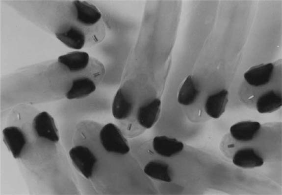
Figure 6.1. Half-length “Coded Wire Tag” implanted into 37-mm-long pink salmon fry (Oncorhynchus gorbuscha.). (Courtesy of Northwest Marine Technology, Inc.)
It is also possible to construct a table of expected recaptures corresponding to the observed recaptures. Let Sj be the survival rate in year j, and fj (the tag-recovery rate) be the probability a tagged animal is recaptured and the tag reported to the investigator in year j. Then the expected number of tag returns in year j, from animals tagged in year i, is given by (table 6.2)
![]()
if i = j, and

if i < j. In the absence of further information, the parameter fj is uninformative because the fraction of tags returned in a year depends on the amount of hunting or fishing effort, the reporting rate of tags, the extent to which tagged animals survive the tagging operation, and the extent to which tags are retained by the animals. In some cases, tag-induced mortality and tag loss can be considerable.
TABLE 6.1
Lake trout tag-return data from Hoenig et al. (1998a) showing the general structure of a tag-recovery matrix

The logic outlined above can be formalized by considering a moment estimator of the survival rate Si. For two cohorts i and i′ released one year apart (i′ = i + 1), a moment estimate is found as the solution of

Thus, the estimate is

For example, if 844 animals are released with tags at the start of 1961 and 989 animals are released at the start of 1962, and if the recoveries in year 4 of the study (1963) are r1961,4 = 26 while r1962,4 = 56 (table 6.1), then an estimate of survival in 1961 is
![]()
Also, note that the number of recaptures from animals tagged in 1961 and recaptured in 1961 is 49 (table 6.1). The expected number for this cell is R1961 f1961 (table 6.2). Equating the observed and expected recaptures gives 49 = 844 f1961. This gives us an estimate of 49/844 = 0.058 for f1961. This parameter is discussed further in section 6.3.
In practice, parameters are estimated from all of the data by using the method of maximum likelihood. The recaptures from a cohort over time are assumed to constitute a random sample from a multinomial distribution.
TABLE 6.2
Cell probabilities πij for a general Brownie tagging model with I = 3 years of tagging and J = 4 years of recaptures

That is, an animal tagged in year i can be recaptured in year i, i + 1, . . . , J, or not be recaptured at all. Thus, the recaptures from cohort i constitute a sample from a multinomial distribution with J – i + 2 categories. The likelihood function for tagged cohort i is then proportional to

where the cell probabilities, πij, are as in table 6.2. The factor before the product refers to the tagged animals never recovered, and the likelihood for all of the cohorts is simply the product of the likelihoods for each cohort, which are considered independent.
The model represented in table 6.2 is very general in that it allows for year-specific values of both the survival rate and the tag-recovery rate. It may be of interest to construct more restricted models. For example, if fishing or hunting effort has been constant over time, it may be of interest to fit a model with a single survival rate for all years. Similarly, if fishing or hunting effort or tactics changed during the course of the study, it may be of interest to fit a model with one survival rate for the period before the change and another survival rate for the period after. The likelihood is still constructed as in (6.2) but the cell probabilities are defined in terms of the restricted set of parameters of interest. From the above, it is clear that it is possible to fit many related models to a single data set. Modern computer packages make this easy with their computational power and interactive interfaces. A key feature has been the use of the Akaike Information Criterion (AIC) for model selection (Burnham and Anderson 1998) to arrive at a parsimonious model, as discussed in chapter 1.
Important things to note are that (1) the Brownie models enable the estimation of the survival rate (or total mortality rate), but not the components of mortality (harvest and natural mortality); (2) to obtain one estimate of the survival rate it is necessary to tag two cohorts of animals, so that the first estimate of survival can be obtained at the end of the second year of study; and (3) it is not possible to estimate the survival rate in and after the most recent tagging year with this model.
6.2 Assumptions of Brownie Models
The assumptions of Brownie type models are (Pollock et al. 1991, 2001) that
1. the tagged sample is representative of the population being studied;
2. there is no tag loss or, if tag loss occurs, a constant fraction of the tags from each cohort is lost, and all tag loss occurs immediately after tagging;
3. the time of recapture of each tagged animal is reported correctly, although sometimes tags can be returned several years after the animals are recaptured;
4. all tagged animals in a cohort have the same survival and recovery rates;
5. the decision made by a fisher or hunter on whether or not to return a tag does not depend on when the animal was tagged;
6. the survival rate is not affected by tagging or, if it is, the effect is restricted to a constant fraction of animals dying immediately after tagging; and
7. the fate of each tagged animal is independent of that of the other tagged animals.
There are several common problems in tagging studies. Newly tagged animals may not have the same spatial distribution as previously tagged animals, especially if animals are tagged at just a few locations, which leads to failure of assumption 1. Animals of different sizes or ages are tagged and these have different survival rates due to size or age selectivity of the harvest, which leads to failure of assumption 4. Older animals have a different spatial distribution than younger animals (due to different migration patterns or emigration), which leads to failure of the assumptions 1 and 4. Tests for these problems and possible remedies are discussed below.
6.3 Interpretation of the Tag-recovery Rate Parameter
As indicated above, the parameter fj of the Brownie model is a composite parameter. The rate of return of tags (i.e., the fraction of surviving tagged animals that is recovered) can be modeled as fj = θj uj λj, where θj is the probability an animal tagged in year j survives the tagging procedure and retains its tag, uj is the probability a tagged animal alive at the start of year j will be captured in year j, and λj is the probability that an animal recaptured in year j will be reported. The parameter u is often referred to as the exploitation rate. If θj and λj can be estimated, then an estimate of the tag-recovery rate parameter, fj, can be converted into an estimate of the exploitation rate, uj (Pollock et al. 1991).
For example, in section 6.2 there was an estimate of f of 0.058 for 1961. Suppose we have determined that all animals survive the tagging procedure with the tag intact (θ = 1) and that 20% of the hunters or fishers who catch a tagged animal will report the tag (λ = 0.2). Then the exploitation rate in 1961 is estimated to be 0.058/(1 × 0.2) = 0.29.
Estimates of θj can be obtained by holding newly tagged animals in enclosures and observing the proportion surviving with tags intact (e.g., see Latour et al. 2001c). One way to estimate tag-reporting rate is by using high reward tags (Pollock et al. 2001, 2002a). Suppose in a tagging study some tags have the standard reward value while others have a special, high reward. It is assumed that all the high reward tags recovered by fishers or hunters are reported. This implies that the value of the reward provides a powerful incentive to return the tag, and that high reward tags are recognized when encountered, e.g., because of a publicity campaign. If the rate of return of standard tags is one-third the rate of return of high reward tags, this implies the fraction of standard tags that is reported is 1/3 (Henny and Burnham 1976). A variety of monetary reward values can be used so that the rate of return of tags can be studied as a function of the reward value (Nichols et al. 1991). Sometimes investigators release high reward tags after a tagging program has been in existence for a number of years. This is likely to change the behavior of the fishers or hunters so the estimates of harvest rates as well as tag-reporting rates pertain to when there is a high reward tagging program in operation but not to the time prior. Pollock et al. (2001) discuss how to handle this situation.
In some cases the investigator would be better off using only high reward tags, instead of a combination of high rewards and standard rewards, even though this leads to many fewer tagged animals being released (Pollock et al. 2001). In essence, high reward tags provide much more powerful information, so the reporting rate for standard tags must be high to justify their use.
Another way to estimate reporting rate is by using hunting or fishing catch surveys (Pollock et al. 1991; Hearn et al. 1999; Pollock et al. 2002a,b). Suppose 5% of the hunting or fishing activity is observed in a hunter, creel, or port sampling survey or by onboard observers. For example, there might be 12 access points to a hunting area and 100 days of hunting; thus, there are 1200 access point-days of hunting activity of which 60 are randomly sampled. Here, sampling an access point-day means observing all hunters’ kill at the access point on the specified day. Suppose further that 15 tags are recovered by the survey agents. This number of recoveries is converted into an estimate of the total number of tagged animals caught by dividing the number of tagged animals observed in the survey by the fraction of the hunt sampled. Thus, the estimated number of tagged animals caught = 15/0.05 = 300. Then, if hunters report all tags, we would expect to receive returns of 300, consisting of the 15 tags already recovered plus 285 additional tags. If only 95 tags (one-third of 285) are recovered outside of the survey, the tag reporting rate is estimated to be 95/285 = 1/3 (Pollock et al. 1991).
Similar methods using fishery observer programs were developed by Paulik (1961), Kimura (1976), and Hearn et al. (1999), who estimated the number of tags in the catch, and by Pollock et al. (2002b), who combined the estimation of reporting rate with estimation of mortality rates. Suppose there are 30,000 metric tons (mt) of fish landed in a fishery, and observers on boats observe 3000 mt of catch (i.e., one-tenth of the total catch) and recover 12 tags. Then it is estimated that 12/0.1 = 120 tagged fish were caught in the fishery, and it should be possible to recover 120 – 12 = 108 more tags if the fishers reported all tagged animals caught. This method differs from the previous method in that here it is assumed that the catches are known, whereas in the previous method the fishing opportunities (the access point by day combinations) were known.
Another method of estimating tag-reporting rate involves planting tagged animals among a fisher’s catch (in a way that does not alter the fisher’s behavior) and noting the fraction of the tags that is recovered (Costello and Allen 1968; Green et al. 1983; Campbell et al. 1992; Hearn et al. 2003). Hearn et al. (2003) discuss planting tags in one component of a multicomponent fishery.
It is important that planted tags be placed in the catch before any humans examine the catch. This generally means that someone must plant the tagged fish before the crew processes the catch. Otherwise, the study will pertain only to the reporting rate for those steps in the processing of the catch that occur after the tags are planted. This method is unlikely to be useful in recreational hunting and fishing studies because it is almost impossible to plant tags surreptitiously soon after capture.
It is also possible to obtain an estimate of the tag-reporting rate (λj) from the tagging data itself (Youngs 1974; Siddeek 1989, 1991; Hoenig et al. 1998a). In general, the information about reporting rate in the tagging data is very weak. However, tagging studies can be designed to enhance the ability to infer reporting rates from tagging data (Hearn et al. 1998; Frusher and Hoenig 2001).
6.4 Functional Linkage Between the Exploitation Rate and the Survival Rate
An important point is that the exploitation rate is not linked functionally to the survival rate in the Brownie model. For example, from one year to the next, both the survival rate and the exploitation rate estimates could increase. Biologically, this is possible if natural mortality decreases over time. In fisheries studies, it is common to assume that the natural mortality rate is constant (or that it fluctuates randomly and independently of exploitation). In this case it is more efficient to use a model in which increasing exploitation rate implies a reduced survival rate. This property is found in the instantaneous rates models developed by Hoenig et al. (1998a,b) and applied by Latour et al. (2001c) and Frusher and Hoenig (2001). These are discussed below. This aspect of tagging models is controversial. Particularly in wildlife studies, investigators are often hesitant to use a linked model, but Anderson and Burnham (1976) and Nichols et al. (1984a) have suggested that a compensatory model is sometimes warranted.
6.5 Instantaneous Rate Models for Estimating Harvest and Natural Mortality
Under simple competing risks theory, in any instant of time, harvest and natural mortality operate independently and additively. The probability of surviving a given period of time of duration t is related to the instantaneous harvest (H) and natural mortality (A) rates in the period by S = e−(H+A)t. Here, H and A have units of time–1 so that (H + A)t is without units. Note that this relationship holds regardless of the relative timing of the harvest and natural mortality. In fisheries studies, H and A are called the instantaneous rates of fishing and natural mortality, and are denoted by F and M, respectively.
The exploitation rate, u, can be defined as the fraction of the population present at the start of the year that is harvested during the year. It is a function of the harvest and natural mortality rates. The exact functional form depends on the relative timing of the forces of mortality. If harvest and natural mortality operate throughout the year at constant intensity, in what Ricker (1975) calls a type two fishery, then the exploitation rate is
![]()
If all the harvest mortality occurs in a restricted period of time at the beginning of the year (a type I fishery), then
![]()
Hoenig et al. (1998a) presented an approach for modeling exploitation rate as a function of an arbitrary pattern of harvest mortality over the course of a year. However, Youngs (1976) and Hoenig et al. (1998a) found that the computed annual exploitation rate is rather insensitive to the timing of the harvest. Thus, in many cases (6.3) or (6.4) will provide an adequate approximation.
A Brownie model can be converted into an instantaneous rates model by simply replacing the Sj in the Brownie model by exp(–Hj – Aj), and replacing the fj by θλuj, where uj is defined by equations 6.3 and 6.4. Alternatively, the more general formulation of Hoenig et al. (1998a) can be used.
6.6 Diagnostics and Tests of Assumptions
Recently, diagnostic procedures have been developed for evaluating models and testing goodness of fit. Latour et al. (2001b) studied patterns in residuals from Brownie models and instantaneous rates models and found that certain types of failures of assumption give rise to particular patterns in the residuals (table 6.3). For example, the residuals in table 6.4 were obtained by fitting an instantaneous rates model that assumes complete mixing of newly tagged animals to a dataset that was modified to simulate newly tagged animals experiencing a lower mortality rate than previously tagged animals, as might occur if tagging took place in areas far from the main fishing or hunting grounds. The fitted model had θλ fixed at 0.18. A single natural mortality rate, A, was estimated under the assumption that natural mortality is constant over all years. Year-specific harvest rates, H, are estimated. See Hoenig et al. (1998b) for a description of the other characteristics of the model. Note that this causes all residuals on the main diagonal to be negative and all residuals one cell to the right of the main diagonal to be positive.
Latour et al. (2001b) noted that the residuals from the Brownie-type model with time-varying survival and tag-recovery rates are subject to some constraints that do not apply to the instantaneous rates models. Specifically, in the time-varying parameterization of the Brownie models the residuals for the “never seen again” column must always be zero (unless constraints are imposed), the sum of the residuals in a row must be zero, the sum of the residuals in a column must be zero, and the residual for the (1, 1) cell must be zero. If the number of years of tagging (I) equals the number of years of recapture, then the (I, I) cell residual must be zero. The instantaneous rates model is only subject to the constraint that the row sums must be zero. The additional constraints associated with the Brownie model make it difficult to visualize some patterns in the residuals. For example, suppose in year 2 of a study a defective batch of tags is used or an inexperienced tagger is employed. One might expect that the number of returns from this cohort over time would be especially low (assumption 2 is violated). With the instantaneous rates model, this is likely to result in a row of negative residuals (with the never-seen-again cell being positive). With the Brownie model, the fact that the sum of the row residuals (excluding the never seen again category) must be zero implies that there are positive residuals to balance the negative ones. Consequently, it is difficult to detect a bad batch of tags by examining Brownie model residuals. Latour et al. (2001b) suggest examining residuals from an instantaneous rate model even when one is interested in fitting a Brownie model.
TABLE 6.3
Patterns in residuals from Brownie and instantaneous rates models caused by failures of assumption

TABLE 6.4
Table of residuals from the fit of a model that incorrectly assumes that newly tagged animals are fully mixed into the population to the data in table 6.1

Latour et al. (2001a) described procedures for testing whether newly tagged animals are fully mixed with previously tagged animals (assumption 1). This involves examining the spatial distribution of tag returns by cohort. If tagged animals are well mixed into the population, then the fraction of the recoveries in a year coming from any particular region should be the same for all tagged cohorts. This can be tested with a contingency table analysis where rows represent tagged cohorts, columns represent tag recovery locations, and the cells specify how the recoveries from a cohort are apportioned among regions.
Myers and Hoenig (1997) explored whether all animals are equally catchable (assumption 6) by examining rates of returns by the size class of animal, i.e., they estimated a selectivity curve for a fishery. The same approach can be used to study whether the rate of tag return varies by other factor such as the sex of the animal. For example, if 10% of the tagged females are recaptured, then (approximately) 10% of the tagged males should be recaptured if the assumption of equal catchability is met. If this condition is not met, the males and females can be analyzed separately to avoid biased estimates.
6.7 Preventing and Dealing with Failures of Assumptions
Latour et al. (2001c) analyzed a tagging study of juvenile red drum in a South Carolina estuary. A feature of the drum population is that the juveniles remain in the estuary for only a few years. Consequently, two or three years after tagging, a cohort will disappear due to permanent emigration. This phenomenon was evident from the pattern of negative residuals in the upper right corner of the residuals matrix. To deal with this, Latour et al. chopped off the upper right corner of the recapture matrix and added the observations to the column specifying the number of animals never seen again. Suppose, for example, animals are tagged for five years and recovered over a five-year period (as in table 6.1). Suppose also that the residuals for the (row = 1, column = 4), (1,4) and (2,5) cells are negative. Then, for row 1, the recaptures r15 and r14 are added to the number of tags never seen again, thus resulting in a tetranomial (r11, r12, r13 and R1 – r11 – r12 – r13). Similarly, for row 2, the recaptures r25 are added to the never seen again category resulting in a tetranomial (r22, r23, r24 and R2 – r22 – r23 – r24). The likelihood is constructed as before by raising the cell probability to the observed number of recaptures in the cell for every defined cell. The “chop” approach is applicable to both Brownie and instantaneous rates models. It results in a loss of precision (because data are discarded) but it can reduce bias.
Suppose males and females have different survival rates. One solution is to simply conduct two tagging studies, one on each sex. This is a legitimate approach but it is expensive and may not be the most efficient way to proceed. It may be that the female survival and recovery rates are functionally related to the male rates, or that the components of mortality are functionally related. For example, suppose that males and females have a different natural mortality rate but the same fishing (or hunting) mortality rates. The table of expected recaptures for a type 1 fishery when there are I = 3 years of tagging and J = 4 years of recaptures is shown in table 6.5. Note there are twice as many rows as years of tagging. This model has three fishing (hunting) mortality rates and two natural mortality rates. If separate models were fitted to each sex, there would be six fishing (hunting) mortality rates and two natural mortality rates. An example of this approach is provided by Frusher and Hoenig (2001).
Often, the survival rate depends on the age of the animal, which, in turn, may depend on the size of the animal. Thus, heterogeneity of survival rates is caused by variation in size of the animals tagged. Brownie et al. (1985) discuss a model that can be applied to age- or size-structured populations. Suppose animals of age 4 are tagged in year 1 and animals of age 5 are tagged in year 2. Let Rij be the number of animals age i tagged in year j, Sij be the survival rate of animals age i in year j, and fij be the tag recovery rate of animals age i in year j. The expected recaptures for a Brownie model for these two cohorts is shown in table 6.6. The logic of the study design is as follows. In year 1, the 4-year-olds in cohort 1 undergo the survival rate of age 4 animals in year 1. The next year the animals in cohort 1 are age 5; consequently, we tag 5-year-old animals to see the contrast between two groups that differ only in that the first group has experienced one more year of mortality than the second group. If we let rij be the number of recaptures of animals tagged at age i and recovered in year j, the ratio of recaptures from the two cohorts in any recovery year (after the first year) can be used to estimate S41. That is, r42/r52 estimates
TABLE 6.5
Cell probabilities πij for an instantaneous rates tagging model with I = 3 years of tagging, J = 4 years of recaptures, and G = 2 sexes
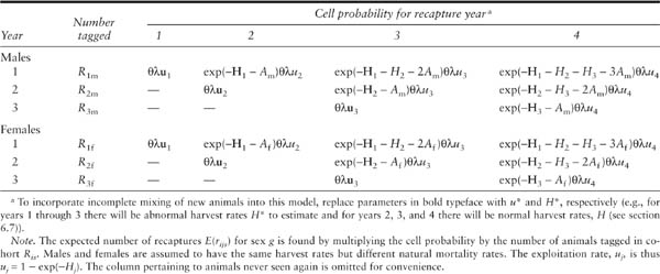
TABLE 6.6
Expected recoveries for an age-structured Brownie model with I = 2 years of tagging and J = 4 years of recaptures


and r53/r63 estimates

This approach can also be used with instantaneous rates models. It essentially requires one to do a separate tagging study for each age group in each year. Again, increased efficiency can sometimes be obtained by modeling the relationships between the age groups. For example, if the fishing gear and fishing tactics remain constant over time, it may be reasonable to assume that the fishing mortality for one age group is a constant fraction of that of another age group (i.e., there is age selectivity). To our knowledge, this has not applied to tag-return models though it is commonly done in the analysis of catch at age data in fisheries assessments.
Perhaps the most critical assumption of a tagging study is that each cohort of tagged animals is representative of the population under study. This implies that all cohorts mix thoroughly with the population so that all cohorts experience the same exploitation rate. However, particularly when animals are tagged and released at just a few locations, the tagged animals may not have time to mix. Ideally, animals should be released at many sites throughout the geographic range of the population, and the number tagged at any site should be proportional to the local abundance at the site. Local abundance is often judged by the catch rate of animals. Using catch rate to assess abundance, however, is reliable only if catch rates are uniform across sampling locations. Assuming that the catch efficiency is uniform among sample locations, tagging 30% of the animals caught in each sample would be appropriate but tagging 30 animals from each sample would not (unless the animals were uniformly distributed over space). If animals can be tagged and released far in advance of the harvest, then the tagged animals will have more time to mix throughout the population. Questions regarding catch efficiency at each location, however, still must be addressed because differences will make it difficult to assess whether representation of tags is geographically proportional.
Hoenig et al. (1998b) presented an instantaneous rates model to handle the situation where newly tagged animals are not thoroughly mixed throughout the population. However, it requires that previously tagged animals (at liberty for at least a year) be thoroughly mixed into the population. The table of expected recoveries for a study of a type 1 (pulse) fishery or hunt with I = 3 years of tagging and J = 4 years of recoveries is shown in table 6.5. Notice that in each year of tagging the newly tagged animals experience a harvest mortality rate of ![]() (the asterisk denotes an abnormal mortality rate, i.e., a rate not experienced by the population as a whole). In contrast, in any recovery year, animals at liberty for more than a year experience the normal harvest mortality rate (assuming they are well mixed into the population at large). Notice also that in each year after the year of tagging, the number of animals available to be caught by the harvesters depends on what happened in the previous year(s). Thus, the cumulative survival rates specified in all cells above the main diagonal have a component of mortality that was abnormal. With this model, it is necessary to estimate I abnormal harvest mortality rates (one for each year of tagging), and J – I normal harvest mortality rates. It is not possible to estimate the normal harvest mortality rate, H1, in the first year of the study because all of the animals in the first year experience the abnormal harvest mortality rate.
(the asterisk denotes an abnormal mortality rate, i.e., a rate not experienced by the population as a whole). In contrast, in any recovery year, animals at liberty for more than a year experience the normal harvest mortality rate (assuming they are well mixed into the population at large). Notice also that in each year after the year of tagging, the number of animals available to be caught by the harvesters depends on what happened in the previous year(s). Thus, the cumulative survival rates specified in all cells above the main diagonal have a component of mortality that was abnormal. With this model, it is necessary to estimate I abnormal harvest mortality rates (one for each year of tagging), and J – I normal harvest mortality rates. It is not possible to estimate the normal harvest mortality rate, H1, in the first year of the study because all of the animals in the first year experience the abnormal harvest mortality rate.
The necessity of estimating the abnormal harvest mortality rates results in a significant loss in precision. Thus, it may well be worth the extra costs associated with dispersing the tagging effort spatially so that a model based on the assumption of proper mixing can be used instead of a model that allows for nonmixing in the year of tagging. Hoenig et al. (1998b) showed that, if a model based on assumed mixing is fitted when a non-mixing model is appropriate, the parameter estimates can be severely biased. However, the estimated standard errors will tend to be small and the analyst may be fooled into thinking that the mortality rates are known precisely when in fact the true values are far from the estimated ones.
To illustrate the importance of accounting for nonmixing, we consider data on lake trout from Youngs and Robson (1975) and modified by Hoenig et al. (1998b). The original data appeared consistent with the assumption of complete mixing, and this was not unexpected given the study design. However, Hoenig et al. modified the number of recaptures along the main diagonal by multiplying them by 2/3 to simulate newly tagged animals having an exploitation rate 2/3 that of previously tagged animals. The number of recaptures in subsequent years were adjusted upward to account for the higher survival rate in the year of tagging. The resulting data are shown in table 6.1.
The fit of the model that assumes full mixing is extremely poor (chi-squared = 34.45, with 9 df, p < 0.0001). The residuals (table 6.4) are all negative on the main diagonal and positive immediately to the right of the main diagonal. On the other hand, the nonmixing model fits well (chi-squared = 7.62, with 5 df, p = 0.18) and there is no pattern to the residuals. For the model assuming complete mixing, the negative of the log likelihood is 1985.3 and six parameters are being estimated. Consequently, the AIC is 2 × 1985.3 + 2 × 6 = 3982.6. For the model assuming nonmixing of newly tagged animals, the log likelihood is 1972.7, the number of parameters is ten, and the AIC is 3965.4. Therefore, the model with nonmixing has the lower AIC and would be selected over the model with complete mixing.
Notice that the estimates from the model assuming complete mixing are very different from those derived from the model allowing for non-mixing in the year of tagging (table 6.7). Also, the standard errors for the nonmixed model are considerably higher than the corresponding standard errors in the fully mixed model. In essence, inappropriate use of the fully mixed model results in biased estimates with misleading standard errors so that they are precisely wrong. The estimates from the non-mixing model are essentially unbiased, and have standard errors that are appropriate and reflect the penalty one pays for having to estimate additional parameters.
Hoenig et al. (1998b) also showed that it may be possible to fit a model that allows for nonmixing to be present during only a part of the year of tagging. This allows more of the tagging data to be used for estimating the normal mortality rates.
Sometimes tagging models have the correct parameter structure but have more variability than predicted under a multinomial model. This would be reflected in reasonable residual patterns but with goodness of fit tests that are highly significant. It has now become standard practice to use variance inflation factors in such situations to adjust the estimated standard errors upward (see chapter 1). Of course, whenever possible, an effort should be made to reduce this problem by tagging few animals at a large number of sites rather than a lot of animals at a few sites.
TABLE 6.7
Model fits to the data in table 6.1

6.8 Chapter Summary
• The logical basis of tagging models (with animals recovered dead) is explained.
• The assumptions required for these models are briefly discussed.
• The interpretation of the tag-recovery parameter in terms of survival, capture, and recovery probabilities is discussed.
• The relationship between the exploitation rate and the survival rate is discussed.
• Models for the estimation of instantaneous harvest and natural mortality rates are discussed.
• Methods for assessing whether assumptions hold and tests for the goodness of fit of models are reviewed, as are approaches for preventing and dealing with failures of assumptions.

Figure 6.2. Bristle-thighed curlew (Numenius tahitiensis), marked with Darvic leg bands and leg flag, Seward Penninsula, Alaska, 1990. (Photo by Robert Gill)