Nine
Examples
9.1 Introduction
In this chapter we provide empirical examples of how to use the models described in earlier chapters to analyze real-world data sets. With numbers rather than symbolic notation, we illustrate some practical aspects of capture–recapture modeling. We provide explicit examples and instructions on the mechanics of model building, and illustrate how to set up analyses in program MARK. We hope that the examples provided in this chapter will reduce the anxiety that often accompanies attempts at new analytical approaches.
Much of this chapter is built around capture–recapture data collected on the European dipper (Cinclus cinclus) (Marzolin 1988). This data set is typical of many capture–recapture studies, and has been analyzed a number of times in the literature (e.g., Lebreton et al. 1992). The dipper data provide a convenient framework for the application of several of the models covered in previous chapters of this book. We start by illustrating how to compute two early and relatively simple capture–recapture models for open populations (Jolly-Seber and Manly-Parr, chapter 3). We then work through a series of more complicated Cormack-Jolly-Seber (chapter 5) analyses of the dipper data using program MARK. We also present an alternative parameterization of the CJS model, in which explanatory covariates are framed in a general regression context. This general regression approach allows capture–recapture data to be analyzed in a familiar and intuitive framework, facilitates complicated covariate structures, and may be more easily understood by newcomers to capture–recapture analysis. Next, we treat the dipper data as if they were collected from a closed population and perform one of the recent approaches to closed-population assessment (i.e., the Huggins model, chapter 4). We then explain how to assess the goodness of fit of a CJS model to the dipper data with parametric bootstrapping. We also estimate the number of dippers using the Horvitz-Thompson population estimator. Finally, we manipulate the dipper data in a way that allows us to illustrate a simple multistate analysis (chapter 7).

Figure 9.1. Steven C. Amstrup gets acquainted with a polar bear cub (Ursus maritimus) on the sea ice north of Prudhoe Bay, Alaska, prior to application of ear tags and lip tattoos. (Photo by Geoff York)
After treatment of the dipper data, we work through a more complicated open-population model (chapter 5) that provides estimates of the number of polar bears in the Southern Beaufort Sea. Finally, we illustrate a dead-recovery analysis in program MARK using data from a study of mallard ducks where tag recoveries were made during 13 hunting seasons (chapter 6).
Although covering only a portion of the depth and breadth of capture–recapture studies, these examples should firm up the reader’s understanding of the what, why, and how of capture–recapture. Hopefully, readers will see similarities between one of these examples and their own data and therefore feel more comfortable about carrying out an analysis.
9.2 Open-population Analyses of Data on the European Dipper
Data from the European dipper study (Marzolin 1988) have been analyzed several times in the capture–recapture literature (e.g., Lebreton et al. 1992; Cooch et al. 1996; Cooch and White 2001; Arnason and Schwarz 1998). The European dipper is a passerine bird that feeds primarily on aquatic insects in montane riparian zones. During seven annual occasions between 1981 and 1987, 294 breeding adult dippers of known sex were captured and marked in an approximately 2200-km2 area of eastern France. Some male and female model parameters are expected to be the same due to the fact that most birds were captured as breeding pairs (Lebreton et al. 1992). Environmental factors such as the flooding or freezing of streams are also known to impact dipper population dynamics, and a major flood did occur in the study area during the 1983 breeding season (Lebreton et al. 1992).
The individual capture histories of European dippers can be presented as

where the seven consecutive 1’s and 0’s indicate whether the bird was captured (1) or not (0) at each sampling occasion, the two “![]() ” represent spaces and were inserted to emphasize their presence in the MARK input file format, a 1 in the next column to the right indicates that the bird is a member of group 1 (males), and a 1 in the last column to the right indicates that the bird is a member of group 2 (females). For example, the capture history 1111000
” represent spaces and were inserted to emphasize their presence in the MARK input file format, a 1 in the next column to the right indicates that the bird is a member of group 1 (males), and a 1 in the last column to the right indicates that the bird is a member of group 2 (females). For example, the capture history 1111000![]() 1
1![]() 0 represents a male dipper that was captured on the first four occasions and not captured on the final three occasions. This is the format of the program MARK input file “DIPPER.INP.” This data file is available at the MARK web site: http://www.phidot.org/software/mark/docs/book/. Table 9.1 presents a condensed version of the entire dipper data set in which the observed capture histories are followed by the number of birds in each group (male or female) that had that capture history.
0 represents a male dipper that was captured on the first four occasions and not captured on the final three occasions. This is the format of the program MARK input file “DIPPER.INP.” This data file is available at the MARK web site: http://www.phidot.org/software/mark/docs/book/. Table 9.1 presents a condensed version of the entire dipper data set in which the observed capture histories are followed by the number of birds in each group (male or female) that had that capture history.
The European dipper data can also be summarized in the form of m-arrays (table 9.2) that list the number of first recaptures from each release cohort. Here Rj denotes the total number of birds captured and released on occasion j (i.e., number in release cohort j), and mjj, denotes the number of birds released on occasion j that were first recaptured on subsequent occasion j′. For example, m12 = 6 in the male m-array contained in table 9.2 indicates that, of the 12 male birds released on occasion j = 1, six were first recaptured on occasion j′ = 2. If some of these six were seen again on occasion 3, they are included in the count m23, because they were captured and released on occasion 2 and first recaptured on occasion 3. As another example, m47 = 1 in the male m-array indicates that, of the 39 male birds captured and released on occasion 4, one was first recaptured on occasion 7. Because no dippers were lost on capture, the number of individuals captured and released alive at each occasion (Rj in table 9.2) is identical to the number of individuals captured at each occasion (nj).
TABLE 9.1
Capture histories for 294 European dippers captured between 1981 and 1987 in eastern France

TABLE 9.2
Observed m-arrays for the European dipper data in table 9.1

Recall from chapter 3 that the distinction between the CJS and the JS models is that the CJS model is conditioned on first capture. Therefore, the parameters estimated by CJS models apply only to the subset of animals that were captured at least once. The main parameters of the CJS model are ϕ and pj where ϕj is the apparent survival probability of animals alive just after capture occasion j to capture occasion j + 1, and pj is the probability of capture on occasion j. The ϕj parameters of the CJS model are referred to as apparent survival probabilities because they do not differentiate between death and emigration.
The JS and Manly-Parr models, unlike the CJS model, assume that all animals in the population have the same probability of being captured as those that actually were captured. The JS and Manly-Parr models therefore permit the estimation of parameters related to the entire population, such as the abundance at occasion j (Nj) and the number of animals that entered the population (e.g., through birth or immigration) and are available for capture between occasions j and j + 1 (Bj). The following two sections illustrate how to fit closed-form versions of the standard JS and Manly-Parr models to the dipper data. Because these models are straightforward and can be computed by hand, they provide insight into capture–recapture modeling that may be difficult to obtain by using the specialized software that is available for more complicated capture–recapture analyses (e.g., program MARK [White and Burnham 1999], program JOLLY [Pollock et al. 1990]).
Jolly-Seber Estimates
To derive JS estimators of survival probabilities, capture probabilities, and abundance (chapter 3), it must be assumed that marked and unmarked dippers were randomly sampled from the population with a constant probability of capture for all individuals at each capture occasion. The JS estimates are functions of the following statistics: the number of animals released alive at occasion j (Rj), the number of animals seen prior to occasion j, not seen at j, and seen again after j (zj), the number of animals released at occasion j and later recaptured (rj), and the total number of marked animals recaptured at occasion j (mj). All of these statistics can be derived from the observed m-arrays. First, rj can be computed as the total of row j. Next, mj can be computed as the total of column j. Finally, zj is the sum of the cells in the rectangular upper submatrix of cell (j − 1, j + 1), i.e., the sum of contents in all cells with a row index less than or equal to j − 1 and a column index greater than or equal to j + 1. For example, z2 is the sum of the upper submatrix of cell (1, 3): z2 = m13 + m14 + ml5 + m16 + m17. The m-array summed over both sexes in table 9.2 yields the following statistics: r1 = 11 + 2 = 13, r2 = 24 + 1 = 25, r3 = 34 + 2 = 36, r4 = 45 + 1 + 2 = 48, r5 = 51, r6 = 52, m1 = 0, m2 = 11, m3 = 26, m4 = 35, m5 = 47, m6 = 52, m7 = 54, z2 = 2, z3 = 1, z4 = 2, z5 = 3, and z6 = 2.
The parameters of biological interest under the JS model (e.g., ϕj, pj, and Nj) can be explicitly estimated by plugging the statistics that were calculated above into equations 3.1, 3.2, and 3.3. Standard errors are calculated by substituting estimated and sample quantities into equations 3.6 and 3.7. For example, ![]() j replaces Nj,
j replaces Nj, ![]() j replaces Mj, nj replaces E(nj), mj replaces E(mj), and rj replaces E(rj) in these equations. Table 9.3 shows the JS statistics and parameter estimates for the pooled dipper data set (males and females analyzed together). Note that this standard JS model allows survival and capture probabilities to vary among occasions, but that because males and females are pooled, differences between sexes are not allowed. Using the nomenclature introduced in chapter 5, this could be described as model (ϕt, pt).
j replaces Mj, nj replaces E(nj), mj replaces E(mj), and rj replaces E(rj) in these equations. Table 9.3 shows the JS statistics and parameter estimates for the pooled dipper data set (males and females analyzed together). Note that this standard JS model allows survival and capture probabilities to vary among occasions, but that because males and females are pooled, differences between sexes are not allowed. Using the nomenclature introduced in chapter 5, this could be described as model (ϕt, pt).
TABLE 9.3
Jolly-Seber estimates of survival and capture probabilities and abundance for the European dipper example

Manly-Parr Estimates
The Manly-Parr model is similar to the JS model in that it estimates parameters related to the entire population (e.g., ϕj, pj, and Nj), and therefore requires the assumption that all individuals have an equal probability of capture on each occasion. The theoretical basis of the Manly-Parr model lies in its intuitive estimator of capture probability (pj). This estimator requires the computation of two statistics: the number of animals known to be alive at each occasion (Cj), and the number of animals known to be alive that were actually captured at each occasion (cj). The estimated probability of capture on occasion j (pj) is simply the ratio (cj/Cj). The statistics Cj and cj cannot be derived from m-arrays, and are most conveniently computed from raw capture histories such as those shown in table 9.1.
We illustrate computation of the Manly-Parr estimated capture probability by considering occasion j = 3. The number of animals known to be alive at occasion 3 (C3) is defined as the number of animals that were caught both before and after occasion 3. For the pooled dipper data set, these animals are represented by the capture histories: 0110110, 0111000, 0111100, 0111110, 0111111, 1101110, 1111000, 1111100, and 1111110. C3 is calculated by summing the frequencies of these histories: C3 = 1 + 2 + 3 + 1 + 2 + 1 + 2 + 1 + 1 = 14. Of the 14 dippers known to be alive at occasion 3, all but one, represented by the capture history 1101110, were actually captured at occasion 3. Consequently, c3 = 13. The Manly-Parr estimate of capture probability is therefore ![]() . The Manly-Parr estimate of abundance at occasion 3 is calculated as
. The Manly-Parr estimate of abundance at occasion 3 is calculated as ![]() . Table 9.4 shows the Manly-Parr statistics and parameter estimates for the pooled dipper data set. As with the JS model, no abundance estimates are available for the first and last occasions.
. Table 9.4 shows the Manly-Parr statistics and parameter estimates for the pooled dipper data set. As with the JS model, no abundance estimates are available for the first and last occasions.
The estimated standard errors that appear in table 9.4 were computed using the equation

TABLE 9.4
Manly-Parr estimates of number of animals known to be alive, capture probability, and abundance from the European dipper data

(Seber 1982, p. 233). The JS and Manly-Parr estimates of abundance and their standard errors are remarkably similar, with an average difference in abundance equal to 0.35 animals.
Cormack-Jolly-Seber Models
The CJS model provides a flexible framework for conditional open-population modeling. Program MARK (White and Burnham 1999) is the most commonly used specialized software for CJS analyses, and provides a user-friendly environment in which CJS (and many other) models can be built that incorporate explanatory covariates. Covariates can be thought of as any additional data (e.g., the size individual animals, yearly weather patterns, etc.) that may help to explain the observed capture histories. In the case of the European dipper, for example, the sex of animals captured and the flood of 1983 are covariates that may help explain variation in survival and capture probabilities, and hence in individual capture histories.
Here we first show how to perform a basic CJS analysis of the European dipper data using the Parameter Index Matrix (PIM) approach of program MARK. The PIMs are the easiest way to build models in program MARK, and allow the specification of simple models in which separate parameters are estimated for different groups (e.g., males and females in the dipper example). We then illustrate how to model the dipper data using the design matrix approach in MARK. Parameter constraints, confounded parameters, and reduced models are the main topics of this section. Our goal is not to present a comprehensive analysis of the dipper data (see Lebreton et al. 1992; Cooch and White 2001), but rather to use real data to illustrate the mechanics of running models and interpreting output in program MARK. We complete the CJS treatment of the dipper data by introducing a general regression approach to modeling capture recapture data. This general regression approach facilitates dealing with complex covariate structures, and is a flexible and intuitive alternative to the design matrix approach used in program MARK.
USING PROGRAM MARK
To begin analyses, start MARK and create a new project by selecting New from the File drop-down menu. Name the project and use the Click to Select File button to locate the DIPPER.INP input file and confirm that it is formatted correctly using the View File button. Designate a CJS analysis by selecting Recaptures Only from the radio-button list to the left. Specify 7 sampling occasions and 2 attribute groups. Click the Enter Group Labels button and enter Males for Group 1 and Females for Group 2. Click OK in the Enter Specifications for MARK Analysis window to read the data into MARK and begin the analysis.
Many mark–recapture analyses begin with the construction of a global model, which is a general model that has a relatively large number of parameters and is thought to be consistent with known biology and causal relationships. A global model for the dipper data is one that allows capture and survival probabilities to vary by year (t) and by sex (s). Using the nomenclature of Lebreton et al. (1992), this model is denoted (ϕs*t, ps*t).
Model (ϕs*t, ps*t) can be fitted using the default PIMs in MARK. PIMs are triangular matrices used to specify the number of parameters that will be estimated in a model. After reading the dipper dataset into MARK, the PIM for the apparent survival of males is automatically displayed. The default PIMs created by MARK for the other parameters can be opened by selecting Open Parameter Index Matrix from the PIM dropdown menu on the main toolbar, clicking the Select All button on the right, and clicking OK. There are a total of 4 PIMs for a two-group CJS model, and each PIM represents the structure of one parameter (ϕj or pj) for one group (males or females).
Table 9.5 is a representation of the parameter indexing that MARK uses for the CJS model (ϕs*t, ps*t). There are six survival parameters for each sex, corresponding to the six intervals between the seven sampling occasions of the study. Similarly there are six capture parameters for each sex, corresponding to the six possible recapture occasions. Because the CJS model conditions on first capture, it is not possible to estimate a capture probability for the first sampling occasion. MARK indexes the survival parameters first as 1–6 for males and 7–12 for females. The capture probabilities are indexed as 13–18 for males, and 19–24 for females.
TABLE 9.5
Parameter structure for European dipper model (ϕs*t, ps*t)

TABLE 9.6
MARK parameter index matrices (PIMs) for the European dipper model (ϕs*t, ps*t)

Once this parameterization is understood, the four PIMs shown in table 9.6 should make sense. Column k in the survival PIMs represents the index used by MARK for the survival probability over the interval k. For example, the 1 in the first column of the male survival PIM is the parameter index used for ϕ1, which is the apparent survival probability of male dippers from occasion 1 to occasion 2. Similarly, column k in the capture PIMs represents the index used by program MARK for the capture probability at occasion k + 1. For example, the 21 in the third column of the female capture PIM is the parameter index for p4, the capture probability for female dippers at occasion 4. MARK sets things up this way because the survival probability can be estimated for the first interval (ϕ1), but the first capture probability that can be estimated is for the second occasion (p2). Studying the PIMs and the parameter structure in table 9.5 should clarify this distinction. Note that in this example, the parameter indices are constant in any given column. This means that neither survival nor capture probabilities are allowed to vary by age of the animals or the cohort into which they were born.
It is important to realize that the numbers in the PIMs are simply indices that MARK uses to keep track of the parameters that are estimated by the model. For example, if you believe that survival does not change with time and want MARK to estimate a single survival parameter for the entire study, the same index value should be entered in every column of the survival PIM. Similarly, if you want MARK to estimate the same capture probability for each occasion of a study, the same index should be entered in each column of the capture PIM. Variation in survival or capture probabilities among cohorts (e.g., if a particular year-class had consistently poor survival because of poor nutrition in its natal year) can be modeled by using different row indices. If animals were assumed to have different survival rates following their first capture, the lower diagonals of the survival PIMs would have indices that differ from those in the remainder of the columns. See Cooch and White (2001) for a more detailed explanation of the use of PIMs.
Because no modification of the default PIMs is required in the current example, model (ϕs*t, ps*t) can now be run. Select Current Model from the Run drop-down menu at the top of the screen. This opens the Setup Numerical Estimation Run window. Specify the name of the current model as Phi(s*t)p(s*t), and then click OK to Run without changing any of the default selections. The Results Browser window now displays a single row with the name of the current model and six other columns of information that are the basis for comparison among models. These will be considered later. Results for the current model are accessed through the buttons at the top of the Results Browser window. To open a Notepad window containing the real parameter estimates (the estimates of the capture and survival probabilities) and associated standard errors, click the fourth button from the left, View estimates of real parameters in Notepad Window. The results should be identical to those shown in table 9.7.
Two aspects of the results shown in table 9.7 require additional explanation. First, the estimate of p3 for males is stated to be 1.000 with a standard error of 0.000. Program MARK often returns parameter estimates of 0 or 1 with corresponding standard errors that are very large or very small. In general, the user must assess such results with care. Parameter estimates that are either 0 or 1 could be caused by some aspects of the data (e.g., sparseness or structural features), which prevent an otherwise estimable parameter from being calculated. Alternatively, the parameter in question could be inherently confounded with another parameter (see below), in which case, it cannot be estimated. In the case of the male capture probability, p3, the estimated value of 1.000 simply means that, according to the data, all of the males that could have been captured at occasion 3 were captured. This subject will be visited later, when alternative methods for specifying model (ϕs*t, ps*t) through the design matrix are discussed.
The second aspect of the results in table 9.7 requiring clarification is that MARK also returns standard error estimates that are either extremely large or 0 for parameters that cannot be estimated. This is apparent in the estimates of ϕ6 and p7 for both males and females. Under the fully time-dependent CJS model, the terminal survival and capture probabilities are confounded and therefore cannot be individually estimated. Program MARK apparently handles this by returning the product of the terminal survival and capture probabilities. For example, the value of 0.7638 for male dipper parameters ϕ6 and p7 actually represents the product (ϕ6*p7). This product cannot be separated into its component survival and capture probabilities.
TABLE 9.7
Survival rate and capture probability estimates from model (ϕs*t, ps*t) for the European dipper data

An additional caveat is required concerning the standard errors that program MARK estimates for the confounded terminal survival and capture probabilities. The magnitudes of these standard errors are not biologically or statistically meaningful. They also can vary depending on the model parameterization or even the format in which the data are read into program MARK. For example, the dipper input file containing individual capture histories (DIPPER.INP) was used to generate results in table 9.7. The standard errors for all of the confounded parameters in this table have a value of 0.000. If the exact same model is specified through the PIMs, but the condensed version of the dipper capture histories (table 9.1) is used, the standard errors for the confounded parameters are very different. For males, the standard errors of ϕ6 and p7 are 162.851, for females the standard errors of ϕ6 and p7 are 70.181. The point here is that the user must be aware of which parameters are confounded before running a specific model. The standard errors estimated by MARK for these parameters should be interpreted as flags that help to point out identifiability problems, not as biologically meaningful values. Chapter 4 of Cooch and White (2001) discusses this issue in more detail.
THE DESIGN MATRIX APPROACH IN PROGRAM MARK
Now we consider two methods for analyzing the dipper data via the design matrix in MARK. The first method builds on the CJS model previously specified through the PIMs, following the analysis presented in chapter 7 of Cooch and White (2001) but with minor modifications to improve the way that parameters are estimated. The second method uses a reformatted version of the dipper data and builds a design matrix based on individual covariates. We present this second method for two reasons. First, basing the analysis on an individual covariate (in this case the covariate sexi to code for the sex of each animal i) presents a useful technique that is easily generalized to other individual covariates. Second, basing the analysis on an individual covariate provides a smooth transition to the general regression approach to capture–recapture, which is described later in this chapter.
The default design matrix for a given model is determined by the parameter structure that is specified in the PIMs. This design matrix can then be modified to create more complex parameter structures than are possible through the PIMs alone, such as models incorporating multiple covariates or additive effects. For a comprehensive treatment of the design matrix, the reader is referred to chapter 7 of Cooch and White (2001).
Continuing the dipper analysis, return to the same MARK project used in the PIM example, and open the default design matrix for model (ϕs*t, ps*t) by selecting Full from the Design pull-down menu at the top of the screen. This design matrix is reproduced here as table 9.8A.
TABLE 9.8A
The MARK default design matrix for the European dipper model (ϕs*t, ps*t)

Table 9.8A can be viewed as a direct representation of the linear equations used to model survival and capture probabilities. In other words, the design matrix expresses the CJS parameters that we are interested in (ϕj and pj) as linear functions of beta coefficients. Each row k of the design matrix corresponds to the real parameter (ϕj or pj) with index value k, as specified in the PIMs. For example, row 9 of the design matrix in table 9.8A corresponds to the parameter with index value of 9, which is the female survival probability ϕ3. The columns of the design matrix correspond to the beta coefficients used to model survival and capture probability parameters. For example, row 9 of the design matrix in table 9.8A shows that the female survival parameter ϕ3 is modeled by the beta coefficients B1 and B5. This means that the linear equation for the female parameter ϕ3 can be written as
![]()
where logit(ϕ3) is a transformation of ϕ3 that is discussed in more detail later, and B1 and B5 are the actual beta coefficients that program MARK will estimate and then use to back-calculate ϕ3. Here B1 is a constant, or intercept, term on which all survival probabilities are based, and B5 is a time effect particular to survival over the third interval. As another example, the male dipper capture probability p2 (the probability of capture at occasion 2) has an index value of 13, and therefore corresponds to row 13 of table 9.8. The linear function for the male parameter p2 can be written as
![]()
The beta coefficients on the right-hand side of this equation correspond, in order, to a constant term for capture probabilities, a general effect for males, a time effect particular to the second sampling occasion, and an effect for males that is specific to the second sampling occasion.
Rows 1–12 of the design matrix represent the equations for the 12 survival probabilities under model being considered, while rows 13–24 represent the equations for the 12 capture probabilities. In effect, the design matrix in table 9.8A represents the same model as was defined earlier using the PIMs (table 9.6). The only difference is that the design matrix presents model (ϕs*t, ps*t) in a regression context, and provides the flexibility inherent in modeling each parameter as a linear function of some combination of products of beta coefficients and covariate values.
For those readers familiar with regression problems, it is instructive to point out that the design matrix in table 9.8A can be summarized by two general regression models. The probability of survival for every animal i between occasion j and j + 1 (ϕij) can be written as

where ln represents the natural logarithm, the B’s are beta coefficients, tia is a dummy variable coding for occasion such that tia = 1 if j = a and tia = 0 if j ≠ a, and sexi is an individual covariate coding for sex such that sexi = 1 if animal i is a male and 0 if animal i is a female. The general regression model for capture probability has the same form but involves different beta coefficients:

The function ln[x/(1 − x)] that appears on the left-hand side of the above equations is called the logit function. This is one of several link functions that are used to model probabilities as linear functions of covariates. Among other things, the logit function ensures that the estimated probabilities are constrained to values between 0 and 1. McCullagh and Nelder (1989) give a general description of these functions and their uses.
Unfortunately, the issue of confounded terminal parameters discussed earlier causes a problem with the default parameterization of the design matrix in MARK (table 9.8A). Consider the terminal survival parameter for females (ϕ6), which corresponds to row 12 of the design matrix and is a linear function of the single beta coefficient B1. B1 also serves as the constant, or intercept, beta coefficient in the linear equations for all of the other survival parameters. Similarly, the terminal capture parameter for females (p7) is a linear function of the beta coefficient that serves as the constant for the capture probability equations, B13. The problem, alluded to earlier, is that under the fully time-dependent CJS model the beta coefficients B1 and B13 are confounded, and only their product can be estimated. Because the MARK default design matrix establishes B1 and B13 as the constant terms in all of the linear equations, the lack of identifiability in those terminal parameters affects the estimation of all of the other beta coefficients. The result is that estimates for B1 to B24 appear reasonable, but have ridiculously large standard errors. This problem can be overcome by changing the parameterization of the default design matrix in table 9.8A so that the beta coefficients that serve as the constant terms can be estimated. The modified design matrix in table 9.8B specifies the same model (ϕs*t, ps*t), except that with this parameterization, the constant term for survival probabilities (B1) corresponds to the female survival parameter ϕ1 (row 7 of the design matrix), and we can individually estimate ϕ1. Similarly, the constant term for capture probabilities (B13) now corresponds to the female capture parameter p2 (row 19 of the design matrix), which can also be individually estimated. Consequently, the other beta coefficients (except for the terminal values) B1 to B24 as defined in table 9.8B can now be estimated and have reasonable standard errors.
With the design matrix in table 9.8B open in program MARK, run the current model by selecting Run from the Run drop-down menu at the top of the screen. The results including the AIC, Deviance, etc. are displayed in the Results Browser: Live Recaptures (CJS) window. The estimates for the beta coefficients B1 to B24 are shown in table 9.9. Notice that under the current parameterization the beta coefficients B7, B12, B19, and B24 are confounded and cannot be individually estimated, as indicated by the very large standard errors. In addition, the beta coefficient B20 has a very large estimate, with an even larger standard error. This relates back to the fact that program MARK is trying to make p3 for males equal to one, which is equivalent to making B20 infinite. The estimates of the real parameters (survival and capture probabilities) for the design matrix in table 9.8B are identical to the estimates from the PIM approach in table 9.7, with the exception of the confounded parameters (ϕ6 and p7 for both males and females).
THE INDIVIDUAL COVARIATE APPROACH IN PROGRAM MARK
We now build a design matrix for model (ϕs*t, ps*t) using the individual covariate sexi. This requires a slightly reformatted version of the dipper input file, which is available as DIPPER_S.INP at http://www.west-inc.com. The first 5 of the 294 individual capture histories in this file look like where again the “![]() ” characters emphasize the spaces required in the MARK input file.
” characters emphasize the spaces required in the MARK input file.

TABLE 9.8B
An alternative parameterization of the design matrix for the European dipper model (ϕs*t, ps*t)

TABLE 9.9
Estimates of beta coefficients for the alternative parameterization of the design matrix for the European dipper model (ϕs*t, ps*t), as shown in table 9.8B

The first 7 digits on each line are the observed capture histories, the next digit (after the space) is the frequency of the history (all 1’s in this example), and the last digit is the individual covariate sexi, which is 1 for males and 0 for females. Start and name a new project in MARK, select the input file, and specify 7 occasions. Leave the number of attribute groups at the default value of 1 and specify 1 individual covariate. Name the covariate by clicking the Enter Ind. Cov. Names button and typing “sex”. Click OK on the Enter Specifications for MARK Analysis window to ingest the data and start the analysis.
The most obvious way to set up the design matrix for model (ϕs*t, ps*t) using the individual covariate sexi is shown in table 9.10A. This parameterization is analogous to the design matrix in table 9.8A, which was the MARK default when modeling two groups. Unsurprisingly, the design matrix in table 9.10A leads to the same identifiability problems in the beta coefficients as discussed above. Once again, the solution is to use a slightly modified version of the design matrix in table 9.10A, which avoids these problems. The preferred way to set up the design matrix for model (ϕs*t, ps*t) using the individual covariate sexi is shown in table 9.10B.
To set up this design matrix, select Reduced from the Design dropdown menu at the top of the screen, specify 24 covariate columns, and click OK. Fill in the blank design matrix so that it looks like table 9.10B. It is important to be comfortable with the fact that the design matrix in table 9.10B specifies the same model as the design matrix in table 9.8B. The reason that the two design matrices look different is that table 9.8B split the dippers into two groups, using one row to represent the linear equation for each male parameter at sampling occasion j, and one row to represent the linear equation for each female parameter at sampling occasion j. Table 9.10B condenses table 9.8B by incorporating the individual covariate sexi, which assumes the value of 0 or 1, depending on the sex of each individual. Hence, a single linear equation (and therefore a single row in the design matrix) is used to represent both male and female parameters at sampling occasion j. It may help to write out the equations for several parameters as specified by tables 9.8B and 9.10B.
One more step is required before running the analysis with the design matrix in table 9.10B. By default program MARK standardizes individual covariates to have a mean of 0 and a range of approximately −3 to +3. Because it does not make sense to standardize a binary sex covariate, uncheck the box Standardize Individual Covariates in the Setup Numerical Estimation Run window. Name and run the model by clicking the OK to Run button at the bottom right.
The design matrix of table 9.10B yields the beta coefficient estimates in table 9.11. Note that although most of the coefficient estimates match those in table 9.9, the point and interval estimates of the confounded parameters are different. At this point there are two methods of obtaining estimates for the survival and capture probability values in which we are ultimately interested. Which of these methods is more convenient will depend on the complexity of the analysis. The first way is to calculate survival and capture probabilities by writing out the linear equations for each parameter using the beta coefficients from table 9.11. For example, the equation for the survival of females between occasions 4 and 5 is
TABLE 9.10A
The design matrix for the European dipper model (ϕs*t, ps*t) using the treatment coding scheme and the individual covariate sexi (0 = females and 1 = males)

TABLE 9.10B
An alternative parameterization of the design matrix for the European dipper model (ϕs*t, ps*t) using the “treatment” coding scheme and the individual covariate sexi (0 = females and 1 = males)

TABLE 9.11
Estimates of beta coefficients for the alternative parameterization of the design matrix for the European dipper model (ϕs*t, ps*t) using the “treatment” coding scheme and the individual covariate sexi (0 = females and 1 = males), as shown in table 9.10B


Solving this equation by taking the inverse of the logit function gives
![]()
which is equal to the estimate derived by the PIM approach in table 9.7. Similarly, the estimated probability of capture for males at occasion 6 is
![]()
which again agrees with the estimate in table 9.7.
To calculate the standard errors of estimated survival or capture probabilities we use the following Taylor series approximation:

where ![]() is the estimated survival or capture probability of interest, p is the total number of coefficients estimated in the model, xi is the value of covariate i that went into the prediction of
is the estimated survival or capture probability of interest, p is the total number of coefficients estimated in the model, xi is the value of covariate i that went into the prediction of ![]() , and cov(Bi, Bj) is the covariance between the ith and jth estimated coefficients. The covariances among model coefficients are available from program MARK through the drop-down menu sequence: Output | Specific Model Output | Variance-Covariance Matrices | Beta Estimates.
, and cov(Bi, Bj) is the covariance between the ith and jth estimated coefficients. The covariances among model coefficients are available from program MARK through the drop-down menu sequence: Output | Specific Model Output | Variance-Covariance Matrices | Beta Estimates.
The second way to obtain point and error estimates of survival and capture probabilities for models using individual covariates is to tell MARK the specific combinations of covariates that identify the real parameter estimates in which we are interested, and then rerun the model. This is done by selecting the User-Specified Covariate Values option at the bottom right of the Setup Numerical Estimation Run window and then clicking the OK to Run button. MARK then prompts the user to specify the individual covariate values of interest. After running the model, real parameter estimates corresponding to the specified covariate values can be accessed from the Results Browser window. This method can be tedious for complex models because it provides real parameter estimates for only one combination of covariates at a time. A model with three binary individual covariates, for example, has 32 possible combinations of individual covariates. That model would have to be run nine times if the researcher was interested in the real parameter values for all possible covariate combinations.
REDUCED MODELS USING THE DESIGN MATRIX APPROACH IN PROGRAM MARK
The MARK analysis of the dipper data to this point has focused on different ways to set up and run the general model (ϕs*t, ps*t). The next logical step in a thorough analysis of these data would be to construct a meaningful set of candidate models. Candidate models are usually less parameterized versions of the global model, each of which represents a biologically plausible scenario. Comparisons among restricted models are intended to evaluate biological hypotheses and may reveal which effects are supported by the data. The models constructed thus far suggest that the data do not support a significant interaction between sex and time effects. The fact that the confidence intervals for the beta coefficients B8–B11 and B21–B23 in Table 9.11 all contain zero indicates that their inclusion in the current model is not justified. It would probably be necessary, however, to build and compare more candidate models using a model fit statistic such as deviance or AIC before concluding that sex has no effect on the time-varying dipper parameters and before deciding on a final model.
The final CJS analysis we would like to show in MARK is use of a design matrix to build a reduced-parameter model. Other authors (e.g., Lebreton et al. 1992) have proposed that the flood experienced in the study area in 1983 affected dipper survival probabilities in the periods 1982–83 and 1983–84. A large variety of reduced-parameter models can be built to investigate this type of hypothesis. A reasonable model for the purpose of illustration is (ϕflood, p.). This three-parameter model does not include sex effects, but allows survival probability to assume one value in the flood years and another value in the nonflood years. It also constrains the capture probability to be constant across all occasions. Continuing in the same MARK project, select Reduced from the Design drop-down menu in program MARK. Specify three covariate columns, click OK, and modify the design matrix to look like table 9.12. By now the equations represented by this design matrix should be apparent. For example, the linear equation for those survival probabilities affected by the flood ![]() can be written
can be written
![]()
TABLE 9.12
The MARK design matrix for the European dipper CJS reduced-parameter model (ϕflood, p.)

where the baseline dipper survival probability is modeled by the beta coefficient B1, and the additive effect of the flood is modeled by B2. Capture probabilities are modeled by the single beta coefficient B3.
Running the design matrix in table 9.12 results in a model with a deviance of 660.1, an increase of only 6.15 from the fully sex- and time-dependent model (ϕs*t, ps*t), even though the two models differ by 21 theoretically estimable parameters. The AIC for the model (ϕflood, p.) is 32 lower than for model (ϕs*t, ps*t). According to the AIC model fitting philosophy of Burnham and Anderson (1998), model (ϕflood, p.) should therefore be considered “better” than model (ϕs*t, ps*t). Keep in mind that applying other model selection methods (e.g., likelihood ratio tests, or Wald t statistics to assess significance of individual coefficients) to some set of candidate models including these two models may not lead to the same conclusion. With this caveat in mind, it will be assumed here that model (ϕflood, p.) is the more useful representation of the dipper data.
Under model (ϕflood, p.) the estimated apparent survival probability for all dippers drops from 0.6071 in nonflood years to 0.4688 in flood years. A capture probability of 0.8998 is estimated for all occasions. Standard errors for model (ϕflood, p.) are reduced because more data are available to estimate a common value when parameters are constrained to be equal, and the apparent precision of that value is increased. We emphasize the word “apparent” here because the tightening of confidence intervals that results from constraining parameters may simply reflect the limitations imposed by the constraining assumptions. And those assumptions (e.g., no variation between sexes) may or may not be valid or reflect biological reality. Although AIC is generally considered a reasonable method of evaluating the trade-off between the apparently higher precision and increased level of bias in a reduced-parameter model, practitioners must appreciate that this trade-off is occurring and the particular way in which it is measured by AIC. While valid model results cannot be ignored, it is ultimately up to the biologist to decide whether assumptions and estimates that otherwise appear statistically appropriate are biologically sensible. Furthermore, statistics may be of little use in detecting departures from biological reality. For example, AIC cannot detect when a biologically important covariate or model form is missing from a larger set of models.
THE GENERAL REGRESSION APPROACH TO CJS MODELS
Although users can delve into the MARK design matrices and reconstruct the regression equations they represent, the process can be awkward and unintuitive. We believe it is conceptually more straightforward to start out by visualizing capture–recapture estimates in a general regression context. This approach involves assuming that the capture and survival parameters we wish to estimate are all functions of chosen covariates. To estimate the real parameters (the capture and survival probabilities), we simply estimate the coefficient values for each covariate and use them for prediction. Going directly to the regression equations can help to eliminate the black box feel of MARK and other programs in which the investigator is forced to work through intermediate steps (such as PIM or design matrices) to get to the underlying equations for the model being assumed.
When capture–recapture problems are framed this way, one matrix represents each covariate. Rather than adjusting elements in PIM and design matrices, the analyst needs to remember only that the rows in each matrix correspond to the animals (index i), and columns correspond to the capture occasions (index j). The matrix representing each covariate can then be thought of as a new page in a three-dimensional array (index k for the 3rd dimension), as illustrated in figure 9.2.

Figure 9.2. Pictorial representation of the three-dimensional array of covariates used to parameterize capture–recapture models. Dimension 1 (rows) represents individual animals. Dimension 2 (columns) represents capture occasions. Dimension 3 (pages) represents covariates.
As an illustration, the flood model, (ϕflood, p.), for the dipper data fit in the previous section would need 2 matrices of covariates in the survival model, and 1 matrix of covariates in the capture model. One matrix in each model would be the intercept and is nothing but a 294 × 7 matrix of 1’s. The second covariate in the survival model would be the flood variable matrix that has all 1’s in columns corresponding to capture occasions 2 and 3. The first 5 rows of the flood covariate, corresponding to the first 5 capture histories (listed above), would be

Although it was not fitted in the previous example, a sex effect could be included in model (ϕflood, p.) by constructing and including a sex effect matrix with element ij equal to 1 if animal i was a male, and 0 if animal i was a female. If a sex effect was desired in either the survival or capture probability model, the sex covariate matrix corresponding to the first 5 capture histories (see p. 214) would be

Time (occasion) effects could also have been included using a combination of covariate matrices, named t1 through t7, that have all 1’s in the column corresponding to the occasion they represent. The time effect matrix for occasion 3 would be

Matrices for interaction effects between sex and time could have been fit and would have had 1’s in cell ij if both the sex and time matrices had 1’s in the corresponding cell. These interaction matrices can be conveniently formed using element-wise multiplication. The interaction covariate matrix for sex and occasion 3 (t3) would have a 1 in column 3 for every male bird that was caught. The first 5 rows of the (t3sex) covariate would be

where “×” denotes element-wise multiplication.
Taken together, the set of all covariates in a capture–recapture model can be thought of as a three-dimensional array, where rows correspond to individuals, columns correspond to capture occasions, and pages correspond to covariates. In contrast to regular linear regression where each covariate value has two subscripts for the row (observation) and column (covariate), each covariate in a capture–recapture problem viewed this way has three subscripts: one for the row (the ith animal), one for the column (the jth capture occasion), and one for the page (the kth covariate). Logistic models for the survival and capture probabilities can then be generically written as

and

where xija and Zija are values of the ath covariate for the ith animal during the jth capture occasion (in the case of capture probabilities) or time interval (in the case of survival probabilities), and βa and γa are unknown coefficients. The capture and survival models for the (ϕflood, p.) model would be

and

To make it easier to conceptualize the problem and to increase the utility of this method, we have, until this point, made no distinction between covariates in the capture and survival models. Rather than complicate the model specification process, we define all covariate matrices to have the same number of columns as capture occasions so that we can write them in either equation. For example, the flood matrix defined above with 7 columns could have been included in either the survival or capture probability model. In reality, however, only 6 columns in each covariate matrix are needed. When a covariate such as flood appears in the survival equation, the last column of its matrix is ignored because there are only k − 1 intervals between occasions when k trap occasions occur. Column j of a survival covariate matrix corresponds to the interval between capture occasion j and j + 1. When a covariate such as flood appears in the capture equation, the first column of its matrix is ignored because the first capture probability is not estimable due to conditioning of the likelihood on first captures.
Specification of very complicated models is straightforward when covariates are viewed as two-dimensional matrices because (1) PIM or design matrices do not have to be manipulated, and (2) most analysts are already familiar with the way regular regression models include complicated terms like interactions, polynomial effects, threshold effects, categorical variables, logarithmic trends, b-splines, etc. The only difference between specifying a complicated model in regular regression and specifying a complicated capture–recapture model is that the variables in the capture–recapture model are matrices instead of columns (vectors).
The general regression approach to capture–recapture modeling using three-dimensional covariate arrays offers distinct practical advantages when modeling individual covariates that can vary over time. As we have shown, the design matrix in MARK allows for specification of CJS models that incorporate time-constant individual covariates. Modeling time-dependent individual covariates in MARK, however, can be quite tedious. Time-dependent individual covariates that indicate membership in different age groups at different times, indicate known changes in reproductive status, or indicate whether an animal is wearing a radio collar can convey a significant amount of information to help explain capture histories. The only difficulty in using time-varying individual covariates is that their values must be known when the animal is not seen. Covariates that must be measured on the animal, such as litter size or herd or group size, cannot be used as time-varying individual covariates. When possible, the general regression approach to capture–recapture analyses offers an intuitive and easy way to incorporate such variables into the modeling process. Time-varying individual covariates simply have varying values in the rows and columns of their matrices.
When comparing complex models with numerous covariates using the three-dimensional matrix formulation, model differences lie entirely in the presence or absence of covariate matrices. Simply adding or subtracting covariates forms different models. Instead of adding or deleting matrices, MARK users construct a new PIM or design matrix every time a covariate is added or removed.
All that is needed to estimate the coefficients in the general capture–recapture regression equations is a computer program that uses the covariate matrices to maximize the statistical likelihood of the data. Program MARK cannot make direct use of the covariate matrices as outlined here. The general regression approach can be carried out using the MRAWIN library of S-Plus or R routines associated with this book (available at www.west-inc.com). Behind the scenes, the MRAWIN routines utilize a Fortran program to maximize the CJS likelihood and compute estimated β and γ coefficients, standard errors, deviances, AIC, and other model fit statistics.
While these routines are free and useful for a wide range of problems, they at present have two important limitations. First, the routines are not developed to the point where they automatically compute the correct number of parameters that can be estimated, as MARK usually does. Computing the correct number of parameters is numerically difficult, and even MARK reports incorrect results with some frequency. When using AIC (or related statistics) for model selection, computation of the correct number of parameters can be a serious limitation because the correct number of parameters needs to be computed by hand. However, if AIC model selection is not being used then knowing the correct number of model parameters is not an absolute necessity. Second, to use these routines, either the S-Plus or R computer package is needed because the capture histories and all covariates need to be read into matrices using regular programming commands. Learning either the S-Plus or R language involves approximately the same amount of difficulty as learning MARK, and once learned S-Plus or R will also be beneficial to analysts for plotting and summarizing their data. The S-Plus and R languages are identical in nearly all respects, but the R package is free and downloadable from the R Project’s web page (www.r-project.org).
If an analyst wishes to use these routines then all that is necessary is to construct the two-dimensional covariate matrices and invoke a single function (named F.cr.estim) specifying the names of the matrices containing capture histories and covariates. The routine F.cr.estim invokes a Fortran routine to do the actual maximization. Using the dipper data and flood matrix indicated above, invoking the following command fits model (ϕflood, p.): fit.dipper.flood<−F.cr.estim(capture=~1, survival=~1 + flood, histories=dipper.histories), where dipper.histories is the name of the 294 × 7 matrix containing the dipper capture histories, and fit.dipper.flood is the name of the fitted capture–recapture model that is returned by the routine. After completion, typing fit.dipper.flood at the S-Plus or R prompt yields the following output:


The deviance, AIC, estimated survival, and estimated capture probabilities are identical with those derived in MARK using the design matrix in table 9.12. For example, the estimated survival of dippers during non-flood years is exp(0.43508)/[1 + exp(0.43508)] = 0.6071, which matches the same result from the previous section.
INDIVIDUAL AND TIME-DEPENDENT COVARIATES IN MARK
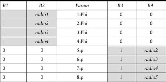
Specifying a model with time-varying individual covariates is complicated using MARK, but it can be done. The MARK user creates a model that incorporates a time-dependent individual covariate by creating a two-dimensional matrix with the appropriate values. Then the user must think of each column of this matrix as a separate individual covariate that applies to a single occasion. In this manner, each time-dependent individual covariate for a study with j occasions can be read into MARK as j separate individual covariates. To avoid confusion and mistakes, the name of each of the j individual covariates should be explicit regarding the occasion to which it applies. Once all of the individual covariates are read into MARK, the design matrix is used to match each individual covariate with its appropriate occasion. The following example should help clarify this approach.
Consider the binary individual covariate radio, which indicates whether or not an animal was wearing a radio collar during some occasions over the course of a five-occasion study. The time-dependent covariate matrix radio has a row for each animal, and five columns. This matrix can be input into MARK by appending it to the individual capture-history matrix (such that row i of the capture-history matrix lines up with row i of the matrix radio) in the .INP file. After starting a MARK project, specify 5 individual covariates in the Enter Specifications for MARK Analysis window, and then name the covariates radio1 through radio5. Table 9.13 shows how these covariates can then be entered into the design matrix to specify the simple example model (ϕradio, pradio), where both survival and capture probabilities vary as a function of the radio covariate over the course of the study. For a short-lived study with only one covariate that varies over time and by individual, this approach in MARK can be effective. On the other hand, it would be enormously tedious in a 30-occasion study in which two or three covariates needed to be handled this way. In the general regression approach, featured in this section, a study including three variables that differed over time and by individual would require the assignment of three covariate matrices. To accomplish the same thing in MARK would require definition of 90 (3 × 30) individual covariates.
TABLE 9.13
The MARK design matrix for the simple example model (ϕradio, pradio), where radio is a time-dependent individual covariate for a 5-occasion study
9.3 The Huggins Closed-population Model Applied to the European Dipper Data
In this section, we violate numerous assumptions and treat the dipper data of table 9.1 as if they came from a closed population so that we can illustrate computation of the Huggins model described in chapter 4. Nobody would consider this a proper analysis of the dipper data, but because the reader is familiar with the dipper data and the data file is already built, it makes an excellent tutorial example. The Huggins approach to modeling closed-population data is very flexible and can be used with many sets of data. We perform one analysis with MARK and another using the spreadsheet program Microsoft Excel. Because the calculations performed in the spreadsheet program are transparent, illustrating the computations that way may help the user to more completely understand the process. Using Excel, however, to complete a real analysis will rarely be feasible.
To fit the Huggins model to the dipper data in MARK, the data file used in the previous example (with one capture history per line) can be used. In MARK, a new project should be started and the Huggins Closed Captures model option chosen. After reading in the data specifying 7 capture occasions, and 2 groups, the default PIM matrix approach would identify full time dependence in the parameters for probability of initial capture and probability of subsequent capture. This default model would estimate a total of 26 parameters, and the reader should be able, by now, to use MARK to complete this most general model by following steps similar to the earlier dipper examples using PIMs.
Here, we want to show how to use the design matrix approach to illustrate modeling original captures as a function of one set of covariates and recaptures with another set of covariates. Sticking to the covariates discussed in earlier dipper examples, we assume that the flood differentially affects recaptures. Therefore, we modify the default design matrix in MARK to incorporate a capture model that includes a sex and time effect, and a recapture model that includes a sex and flood effect. The design matrix for this model is shown in table 9.14. Note that in this example, the sex effect we consider is a simple step effect constant across time. Hence, we are not considering possible interactions between sex and time or between sex and flood effects. Once fitted, this model estimates 141 males (SE = 1.8) and 153 females (SE = 2.3), for a total of 294 birds. Note also that the Huggins model produces only one estimate of the number of birds, not one for each capture occasion. This is because this is a model that assumes the population is not changing during the course of the study. In a real study, each covariate would be investigated for its ability to explain variation in the capture histories. Interactions between sex and time or sex and flood effects would be logical things to examine. Some variables would potentially be removed, while others would potentially be added in this exploration of the data. We will forgo the model-selection process in this example in order to focus on illustrating the underlying calculations and some fundamental ideas of maximum likelihood estimation.
The Huggins model likelihood function is relatively simple and it can be computed and maximized in a spreadsheet program like MS Excel. Although starting the spreadsheet process is a bit awkward, it is very instructive because the transparency of spreadsheet operation illuminates a fundamental idea behind all maximum likelihood techniques. All maximum likelihood techniques maximize a statistical likelihood, and the maximization process can be thought of as taking educated guesses at parameters until a certain function of the data (i.e., the likelihood) is maximized. To fit the likelihood in a spreadsheet, the spreadsheet must have a procedure to find the values in several cells that maximize the value in another cell.
TABLE 9.14
The MARK design matrix used to fit the Huggins closed-population model to the European dipper data

In Microsoft Excel the solver procedure can carry out the maximization. This may need to be installed for the purpose. When using any maximization routine it is best to independently verify that the true maximum was achieved. Some maximization routines have difficulty achieving the correct maximum when the function is complicated. The solver routine in MS Excel is sufficient to find the maximum of the simple Huggins likelihood illustrated here. However, analysts will probably want to use a more general purpose maximization routine on more complicated real-life problems.
We illustrate computation of the likelihood for a simple Huggins model where the initial capture probabilities change on each sampling occasion, as do recapture probabilities (i.e., there are no heterogeneity or covariates). To make this description easier, assume 4 trapping occasions and that the capture histories are contained in columns A–D of a spreadsheet, starting in row 3, as shown in figure 9.3. Also, guesses at the initial probabilities of capture are contained in cells A1, B1, C1, and D1 (more columns will be needed if more occasions are present, and the multinomial expressions described below would also be expanded accordingly if more occasions are present), and guesses at the recapture probabilities are contained in cells B2, C3, and D3. Recall that there are only three recapture probabilities that can be estimated with four sampling occasions. The following formula should be entered into cell E3 and copied down the column:

This calculates the logarithm of the likelihood of obtaining the initial captures, as explained in the Models Incorporating Covariates section in chapter 4. The following formula should then be entered into cell F3 and copied down the column:


Figure 9.3. Spreadsheet used to illustrate computation of the Huggins model. Parameters are in cells A1:D2. Example capture histories are in cells A3:D13. Intermediate calculations necessary to compute the likelihood are in columns E, F, G, and H. The final log likelihood for this data and these particular parameter estimates is in cell H15.
This formula calculates the contribution of the recapture histories to the log-likelihood. Next, the following formula should be entered into cell G3 and copied down the column:
![]()
This calculates the denominator of the Huggins likelihood. Lastly, = E3 + F3 − G3 should be entered into cell H3 and copied down the column. Column H contains the total contribution of each capture history to the log-likelihood. The full log-likelihood can now be calculated by summing all the rows of column H. For the particular set of 11 capture histories and parameter guesses displayed in figure 9.3, the log-likelihood is −29.29, as shown in cell H15. By changing the parameters, we wish to make this number as large as possible.
It is instructive to change the cells in the range A1:D2 (i.e., the parameters) and see how cell H15 changes. If cell H15 gets larger, the change in parameters is in the right direction because the log-likelihood is closer to its maximum. If cell H15 gets smaller, the change in parameters is in the wrong direction.
All that is left to do is continue guessing at the values in cells A1:D2 until the value in cell H15 is maximized. This is where the solver function of the spreadsheet is useful. Basically, the solver asks for a range of cells to change (i.e., A1:D2), an objective cell (i.e., H15), and whether or not to maximize or minimize. Consult the spreadsheet’s help file on proper use of the solver. This model, it turns out, is over parameterized, and multiple maximum likelihood estimates exist for the same likelihood value. A solution set reported by MARK is: P1 = 0.4103, P2 = 0.4174, P3 = 0.4776, P4 = 0.4571; C2 = 0.4, C3 = 0.5, and C4 = 0.4. The maximum likelihood value reported was −29.287. A single solution could be found using more data or different models.
A spreadsheet can easily calculate parameter point estimates as described above. Most spreadsheets, however, cannot easily compute standard errors. Whereas add-in routines for some spreadsheet programs may suffice for calculating variances, the most straightforward estimation of variances for the Huggins model are available from either program MARK or CARE-2 as described in chapter 4.
9.4 Assessing Goodness-of-Fit
How well the full CJS model fits data from each sex can be tested with goodness-of-fit (GOF) statistics. Currently, there are two common GOF methods for assessing whether the arrangement of data meets the CJS assumptions (see chapters 3 and 5). One method involves two chi-squared contingency table analyses called Test 2 and Test 3. The other method involves parametric bootstrapping. Both procedures are available in MARK, and some practical aspects of both will be described here.
Both GOF testing procedures provide two types of information: (1) a goodness-of-fit p value, and (2) an estimate of a variance inflation factor (ĉ). This ĉ is a measure of overdispersion, or the amount of excess variance in the data due to violation of model assumptions. In other words, a model might be built on the assumption that data are arranged according to a Poisson distribution. Lack of independence, heterogeneity, or other unknown features may increase the dispersion of the data (i.e., increase the variance) beyond what would be predicted by a Poisson distribution. The estimated value for ĉ then can be used to correct the model selection criteria for the extra variation above that predicted by the assumed model. When this is done, the analysis changes from a true maximum likelihood analysis into a quasi-likelihood analysis because the data are no longer hypothesized to come from a true likelihood. When ĉ is incorporated into AIC calculations, we label the measure QAIC to acknowledge the quasi-likelihood nature of the statistic.
Both Test 2 and Test 3 compute the expected number of captures in cells of a contingency table based on the model of interest and compare those expected values to the actual number of captures in those cells. Test 2 examines the pattern of recaptures of animals that were captured during a particular occasion, say occasion #3. It contrasts the observed and expected number of animals captured at the first occasion following the one of interest (in this case #4) with the expected number of animals captured on all occasions beyond that next occasion (#5+). We count the total number of first recaptures after occasion j (#3 in this case), and then partition those into the number seen and not seen at occasion j and first recaptured at occasion j + 1. An example from the dipper data will help illustrate. Of the female dippers captured prior to or on occasion 3, 19 of them were later recaptured. Of those 19, 17 were seen at occasion 3 and first recaptured at occasion 4, 1 was seen at occasion 3 and not recaptured until after occasion 4, 1 was not seen at occasion 3 but was first recaptured at occasion 4, and 0 birds were not seen at occasion 3 and first recaptured after occasion 4. These counts for the female dippers recaptured after occasion 3 appear in table 9.15.
TABLE 9.15
Chi-squared contingency table for Test 2 associated with female European dippers and occasion #3

If the CJS model fits, the number of animals in each cell follows a multinomial distribution and the expected count in each cell is simply the product of the two marginal totals, divided by the grand total. In other words, if all animals have the same probability of being captured at each occasion (a simple time-dependent model), then the proportion of animals captured at occasion #3 and again at #4, should be the same as the proportion of animals captured before #3 and at #4. Similarly, the proportion of animals captured at #3 and not captured until occasion #5 or later should be the same as the number of animals captured before #3 and at occasion #5 or later. For table 9.15, the expected count for cell (1, 1) is 18(18)/19 = 17. The expected count for cell (2, 1) is 18(1)/19 = 0.95. Using the observed and expected counts for the cells, the chi-squared statistic for the table can be computed as

where oij, and eij, are the observed and expected counts for cell (i, j), respectively. This statistic approximately follows a chi-squared distribution (with 1 degree of freedom) under the null hypothesis that the CJS model fits. For the data in table 9.15, χ2 = [(17 − 17)2/17] + [(1 − 0.95)2/0.95] + [(1 − 0.95)2/0.95] + [(0 − 0.05)2/0.05] = 0.055.
As with all chi-square tests the approximation to the chi-square distribution may be poor if the expected cell counts are low. An accepted rule of thumb is that the chi-squared statistic is unreliable (i.e., does not follow a chi-square distribution) if any of the expected counts are <2. Because most capture–recapture datasets violate this rule of thumb for at least one or more occasions, chi-square statistics computed occasion by occasion almost always are summed across occasions and groups to compute an overall χ2 statistic.
If the CJS model does not fit, the observed counts will be consistently far from their expected values, and the overall χ2 statistic will be large relative to the chi-square distribution. If the area under the chi-square distribution to the right of χ2 (i.e., the p value associated with χ2) is less than a, we reject the null hypothesis that the CJS model adequately fits the data. The overall Test 2 chi-square statistic for female dippers is χ2 = 3.2503 (df = 4, p = 0.5168), while the overall Test 2 chi-square statistic for both males and females is χ2 = 7.5342 (df = 6, p = 0.2743). Insignificant values for both Test 2 statistics suggest no reason to believe the full CJS model does not fit the data.
Test 3 contrasts the observed and expected number of animals captured at each occasion that were seen and not seen before with those counts of animals that were seen and not seen after each occasion. Again, the idea is that animals captured at one occasion, #3, for instance, should have the same probability of being captured after occasion #3 whether or not they were captured before occasion #3. The Test 3 contingency table for the 41 female dippers captured at occasion #3 appears in table 9.16. The total number of animals in each Test 3 contingency table is the total number of animals seen at occasion j. The expected count in each cell is again the product of the two marginal totals divided by the grand total. The expected count in cell (1, 1) of table 9.16 is 14(18)/41 = 6.15. The expected count in cell (2, 1) is 27(18)/41 = 11.85. Similar to Test 2, an animal group’s contingency tables and chi-square statistics for Test 3 are computed for every occasion and summed to get an overall test of fit. Test 3 for the female dippers is χ2 = 2.0412 (df = 3, p = 0.5639), while Test 3 for both male and female dippers is χ2 = 10.7735 (df = 15, p = 0.7685). As with Test 2, Test 3 does not indicate lack of fit of the full CJS model to the dipper data.
While tedious to compute by hand, Tests 2 and 3 are computed by program Release, which is a component of program MARK. To compute Tests 2 and 3 in MARK, simply read in the data file as above. Go to the “Tests” menu and click Program RELEASE GOF. In the resulting output, all Test 3 contingency tables appear first, followed by all Test 2 contingency tables, followed by a summary of both Tests 2 and 3 together. It is this combined summary table that is usually most interesting because it has the most degrees of freedom (and is therefore most powerful), and it can be used to compute an estimate of ĉ. From the “Goodness-of-Fit Results (TEST 2 + TEST 3) by Group” table that appears in the RELEASE results applied to the dipper data, the total χ2 = 18.31 (df = 21, p = 0.6295). Given the high p value, results of these combined tests, like the results of Test 2 and Test 3, do not indicate lack of fit of the CJS model to the dipper data. Although both Test 2 and Test 3 rely on fairly intuitive assumptions about the distributions of captures and recaptures, they appear to have low power to actually detect a departure from the CJS model (Manly et al. 1999). Low power should be recognized when goodness-of-fit statistics are evaluated, and it suggests that development of other tests to assess model fit may be a fertile area for future research.
TABLE 9.16
Chi-squared contingency table for Test 3 associated with female European dippers and occasion #3

The best and most common estimate of ĉ is calculated from this same table in the RELEASE output file as the overall χ2 statistic divided by degrees of freedom. For the dipper data, ĉ = 18.31/21 = 0.87. It is customary to set ĉ = 1.0 if the actual estimate of ĉ < 1, as in this case. A ĉ ≤ 1, like the GOF tests, suggests no lack of fit and therefore no adjustment to the AIC testing criteria is indicated.
Another intuitively appealing method to assess model fit is called the parametric bootstrap. The parametric bootstrap or simulation procedure uses the parameters from a selected model to create a large number of simulation data sets. Data in these simulation data sets fit the parameters of the selected model and therefore are known to meet all of the assumptions of the model (e.g., homogeneity of capture and survival probabilities). Diagnostic statistics such as the deviance, degrees of freedom, and deviance/degrees of freedom can then be calculated for each of the simulated data sets. The distribution of these diagnostic values computed on the simulation data sets is then compared to the same diagnostic values calculated from the selected model when it is applied to the real data. If the observed diagnostic statistics are abnormal when compared to those generated by the simulated data sets, then a violation of assumptions is suggested. For example, if the maximum deviance computed from 1000 datasets that satisfy all assumptions is 250, but the observed deviance is 400, one can reasonably infer that some assumptions of the model are violated in the real data set. In addition, if the average deviance from 1000 data sets known to satisfy all assumptions is 200, but the observed value is 400, then a reasonable estimate of the amount of the extra variation not accounted for by the model (the variance inflation factor) is ĉ = 400/200 = 2.
For the dipper data, 1000 parametric simulations were performed in MARK with the full CJS model applied to both sexes separately. The observed deviance of the fitted model was 71.5. Comparing this value to the ranked deviances from 1000 simulations revealed that 95 of the 1000 simulated deviances were greater than or equal to 71.5. Thus, the probability of a deviance as large or larger than the observed value is estimated to be p = 0.095. This probability falls short of the commonly used significance criterion of 0.05. Statistical rules aside, a deviance this great gives a suggestion of some violation in the assumptions of the model. This result contrasts with the Test 2 and Test 3 results already reported, and suggests that a search for better fitting models (e.g., by testing different covariates and exploring other assumptions) is in order.
One method to estimate ĉ with the results of parametric bootstrapping is to divide the deviance calculated from the observed data by the mean of the simulated deviances (Manly et al. 1999). For the dipper data, the mean of the bootstrapped deviances is 55.66, and this ratio is ĉ = 71.5/55.66 = 1.28. As with the significance test in the previous paragraph, this estimate of ĉ also indicates some lack of fit between the selected model and the observed data. Estimated values of ĉ can be used to correct Akaike’s information criteria (AIC) for extra variation. When this is done, the AIC becomes a quasi-AIC (QAIC) to reflect the fact that the likelihood with the extra variation is a quasi-likelihood (Burnham and Anderson 1988; chapter 5).
As seen above, the GOF tests and ĉ calculations from bootstrapping differed from those relying on Test 2 and Test 3. The latter suggested no lack of fit and no overdispersion in the data. The bootstrapping results, on the other hand, suggested at least moderate overdispersion and lack of fit. Because corrections for overdispersion will affect parameter estimates provided by the model, this difference is not trivial. As pointed out previously, Manly et al. (1999) reported that Test 2 and Test 3 have low power. White (2002), on the other hand, performed simulations suggesting that bootstrapped estimates of GOF may be unreliable and that Test 2 and Test 3 are preferable. Based on the results of White (2002) and until further investigation of these techniques can be performed, we recommended that ĉ be estimated based on the results of Test 2 and Test 3.
9.5 Horvitz-Thompson Open-population Size Estimates
As pointed out above, one difference between the JS model and the CJS model approach is that the CJS model deals only with the marked component of the population. Because it does not make inference to the unmarked portion the CJS model provides estimates of capture and survival probabilities only. Capture probabilities are, however, related to population sizes. If the investigator is willing to assume that all European dippers in the study area had positive, but not necessarily equal, capture probabilities, then the Horvitz-Thompson estimates of population size given by equation 5.5 can be computed.
Recall that a Horvitz-Thompson estimate is computed as the sum of the reciprocals of the capture probabilities for the individual animals captured on a sampling occasion. For purposes of illustrating the computations, we will apply the Horvitz-Thompson estimator using the capture probabilities shown in table 9.7. We know from the goodness-of-fit tests in the previous section and from previous analyses of the dipper data that the model used to generate the results in table 9.7 does not adequately explain the heterogeneity in the sample. To provide a simple example, however, we ignore that shortcoming, and show how to apply the Horvitz-Thompson estimator as if there were no heterogeneity issues.
Estimated capture probabilities for female dippers range from 0.67 to 0.93; note that p7 is confounded with ϕ6 in this model. Estimated capture probabilities for male dippers range from 0.72 to 1.0. In the model used to generate table 9.7, members of each sex have the same covariate values each sample occasion. Consequently, equation 5.5 reduces to the number of captured males and females divided by their respective capture probabilities. The estimate of population size at time j = 2, …, 6 is therefore

where njF is the number of females caught at time j, and njM is the number of males caught at time j. Both njF and njM can be found in table 9.2.
Substituting the appropriate values, the estimate of population size at time 2, when 26 male dippers and 34 female dippers were captured, is ![]() 2 = 34/0.673 + 26/0.717 = 86.75. Not surprisingly this is virtually identical to the JS population estimate shown in table 9.3. The rest of the Horvitz-Thompson estimates of population size are
2 = 34/0.673 + 26/0.717 = 86.75. Not surprisingly this is virtually identical to the JS population estimate shown in table 9.3. The rest of the Horvitz-Thompson estimates of population size are ![]() 3 = 84.67,
3 = 84.67, ![]() 4 = 87.63,
4 = 87.63, ![]() 5 = 97.4, and
5 = 97.4, and ![]() 6 = 105.15.
6 = 105.15.
The variance of ![]() j can be approximated, assuming that captures of individuals are independent, using Taylor series expansions. The approximation is derived by noting that
j can be approximated, assuming that captures of individuals are independent, using Taylor series expansions. The approximation is derived by noting that
![]()
(McDonald and Amstrup 2001) and approximating each term. The first term on the right-hand side of (9.5) can be decomposed as

Assuming E[![]() ij] = pij (i.e., that
ij] = pij (i.e., that ![]() ij is an unbiased estimate of pij), the “delta method” for approximating the covariance of a function of random variables (Seber 1982, p. 9) involves 2nd-order Taylor series expansions and yields the approximation
ij is an unbiased estimate of pij), the “delta method” for approximating the covariance of a function of random variables (Seber 1982, p. 9) involves 2nd-order Taylor series expansions and yields the approximation

so that,

If a logistic link function is used to relate the covariates to capture probabilities ![]() , where xij is a vector of length p containing covariate values for animal i at capture occasion j and
, where xij is a vector of length p containing covariate values for animal i at capture occasion j and ![]() is the vector of estimated coefficients), then another application of the delta method yields
is the vector of estimated coefficients), then another application of the delta method yields

where ![]() β is the estimated p × p variance-covariance matrix for the coefficients in
β is the estimated p × p variance-covariance matrix for the coefficients in ![]() . Other link functions, such as arcsin, will require different approximations in equation 9.7. The other equations in this section, however, hold for all link functions.
. Other link functions, such as arcsin, will require different approximations in equation 9.7. The other equations in this section, however, hold for all link functions.
If we assume that captures of individuals are independent of one another, and apply the 2nd-order Taylor series approximations.

and

the second term of (9.5) can be decomposed as

Substituting (9.6) and (9.8) into (9.5) yields the approximate variance of ![]() j,
j,

To obtain an estimator of (9.9), we rely on the Horvitz-Thompson theorem and the reasoning behind its proof. When any quantity, say υi, is obtained from a unit that is sampled at probability pi, the Horvitz-Thompson theorem says that an unbiased estimator of ∑N υi is ∑N Iiυi / pi, where Ii equals 1 if unit i was obtained in the sample and Ii = 0 otherwise. The sum in the Horvitz-Thompson theorem is over both sampled and un-sampled units because Ii = 0 for all unsampled units. All terms in the first summation of (9.9) are obtained in the sample from animals captured with probability pij. All terms in the second summation of (9.9) are obtained in the sample with probability pijpi′j because capture of animal i is assumed to be independent of the capture of animals i′. Applying the Horvitz-Thompson theorem and substituting unbiased estimates for the p’s and variances, we obtain the approximately unbiased estimator,

where hij is the jth entry in the capture history for animal i, n is the total number of animals captured, υâr(![]() ij) is an estimate of the capture probability variance for the ith individual at occasion j, and
ij) is an estimate of the capture probability variance for the ith individual at occasion j, and ![]() is an estimate of the covariance in estimated capture probability between animal i and animal i′ at occasion j. Using a logistic link function, we can estimate both
is an estimate of the covariance in estimated capture probability between animal i and animal i′ at occasion j. Using a logistic link function, we can estimate both ![]() from (9.7) since
from (9.7) since ![]() .
.
If we define the coefficient of variation (CV) for the estimated capture probabilities as ![]() the bracketed term in (9.10) becomes
the bracketed term in (9.10) becomes ![]() . This term is a 4th-degree polynomial in
. This term is a 4th-degree polynomial in ![]() and, along with
and, along with ![]() , represents a penalty in variance to be paid for imprecise estimation of capture probabilities. The CV term is small (<1.28) if the CV of estimated capture probability is less than 30%, but is substantial (>5) if CV is greater than 1.0. In cases where capture probabilities are precisely estimated and most CVs are small, it will be reasonable to drop this term. If dropped, the estimator in (9.10) is equivalent to the variance estimators of Huggins (1989), Borchers et al. (1998), and Taylor et al. (2002). McDonald and Amstrup (2001) derived a different variance estimator along these same lines using 1st-order Taylor series approximations, but without the covariance terms. While their estimator is easy to calculate by hand, and is reasonably accurate when capture heterogeneity is small, it will underestimate the variance of population size in many cases. If possible, the estimator in (9.10) should be favored over that of McDonald and Amstrup (2001).
, represents a penalty in variance to be paid for imprecise estimation of capture probabilities. The CV term is small (<1.28) if the CV of estimated capture probability is less than 30%, but is substantial (>5) if CV is greater than 1.0. In cases where capture probabilities are precisely estimated and most CVs are small, it will be reasonable to drop this term. If dropped, the estimator in (9.10) is equivalent to the variance estimators of Huggins (1989), Borchers et al. (1998), and Taylor et al. (2002). McDonald and Amstrup (2001) derived a different variance estimator along these same lines using 1st-order Taylor series approximations, but without the covariance terms. While their estimator is easy to calculate by hand, and is reasonably accurate when capture heterogeneity is small, it will underestimate the variance of population size in many cases. If possible, the estimator in (9.10) should be favored over that of McDonald and Amstrup (2001).
equation 9.10 is complicated and difficult to compute. Fortunately, both 9.10 and 9.10 (without the CV term) are computed by the MRAWIN software package. Running the fully time-dependent CJS model by sex on the dipper data (table 9.1), and requesting that F.cr.estim estimate variances by inverting the Hessian of the maximization, produces the same parameter estimates as in Table 9.7, but slightly different standard error estimates. For male birds, the standard errors estimated by F.cr.estim for capture probabilities were 0.1980, 0.0000, 0.0822, 0.0612, and 0.0601 for ![]() through
through ![]() , respectively. For females, estimated standard errors were 0.2037, 0.1302, 0.0703, 0.0748, and 0.0567 for
, respectively. For females, estimated standard errors were 0.2037, 0.1302, 0.0703, 0.0748, and 0.0567 for ![]() through
through ![]() , respectively. Applying (9.10) to this model resulted in the estimated standard errors se(
, respectively. Applying (9.10) to this model resulted in the estimated standard errors se(![]() ) = 20.23, se(
) = 20.23, se(![]() ) = 7.77, se(
) = 7.77, se(![]() ) = 6.30, se(
) = 6.30, se(![]() ) = 6.39 and se(
) = 6.39 and se(![]() ) = 5.86. Because the estimated CVs of capture probabilities were all <30%, it might be reasonable to apply (9.10) without the CV term. Doing so resulted in the estimated standard errors se(
) = 5.86. Because the estimated CVs of capture probabilities were all <30%, it might be reasonable to apply (9.10) without the CV term. Doing so resulted in the estimated standard errors se(![]() ) = 19.97, se(
) = 19.97, se(![]() ) = 7.74, se(
) = 7.74, se(![]() ) = 6.29, se(
) = 6.29, se(![]() ) = 6.37, and se(
) = 6.37, and se(![]() ) = 5.85. Even though it remains small, the largest difference between these two sets of variance estimates occurs at occasion 2 where CVs are highest.
) = 5.85. Even though it remains small, the largest difference between these two sets of variance estimates occurs at occasion 2 where CVs are highest.
9.6 A Multistate (Multistrata) Model
In this section, we use a modified version of the dipper data to demonstrate a multistate model in MARK. Whereas these models were originally conceived to explain movements of animals among geographic strata, they can explain any change of an animal’s state, as discussed in chapter 8. Multistate models are generalizations of the CJS model, which allow for the movement of animals between states. The state of an animal at each sampling occasion may refer to a geographic location, a physiological state (such as nesting), or any other condition of interest. Data for multi-state models are similar to conventional capture–recapture data. Each animal is represented by an individual capture history indicating whether or not it was encountered at each occasion (e.g., a series of 0’s and 1’s for CJS studies). For multistate models, however, the generic 1 used to designate a capture is replaced by a variable that reflects the state in which the animal was encountered. For example, the multistate capture history “AB0B” describes an animal that was caught at time 1 in state A, was caught at time 2 in state B, was not caught at time 3, and was last caught at time 4 in state B.
For the purposes of this example, the dipper data set was transformed into an artificial multistate data set by randomly assigning each capture to either state A or state B by flipping a coin. No distinction is made between the two groups (male and female) for this example, and therefore each individual capture history is followed by a single 1 to represent its frequency. The first 5 lines of the 294 modified individual capture histories look like

Because the designation of states was random, there are roughly as many captures in state A as in state B at each occasion, and we therefore expect that the probabilities of transition between the two states (ψAB and ψBA) estimated by MARK will be close to 0.5. The modified dipper data set was read into MARK specifying the Multi-strata Recaptures only data type, 7 encounter occasions, 1 attribute group, and 2 strata.
The three fundamental parameters in a multistate model are defined as follows: ![]() is the probability that an animal in state A at sampling occasion i survives and remains in the study population until sampling occasion i + 1,
is the probability that an animal in state A at sampling occasion i survives and remains in the study population until sampling occasion i + 1, ![]() is the probability that an animal alive in state A at time i is captured, and
is the probability that an animal alive in state A at time i is captured, and ![]() is the probability that an animal is in state B at sampling occasion i + 1, given that the animal was in state A at period i and that it survived until i + 1 and remained in the study population. To illustrate the mechanics of running a multistate model in MARK, we consider a simple model which assumes that the probabilities of survival, capture, and transition are constant within each state for the duration of the study, but are different between the two states. An appropriate name for this model is (Sspsψs), where the superscript s denotes the fact that parameters are allowed to vary by state. Model (Sspsψs) has 6 independent parameters: SA, SB, PA, PB, ψAB, and ψBA. The structure of these parameters is represented by 6 PIMs in program MARK. To specify model (Sspsψs), a single index value is entered into each of the 6 PIMs. For example, all values in the survival PIM for state A are set to 1, all values in the survival PIM for state B are set to 2, all values in the capture PIM for state A are set to 3, and so on. The structures of all of the PIMs for model (Sspsψs) are shown in table 9.17. The reader should be aware that, as with other types of capture–recapture modeling in program MARK, it is possible to fit more complex multistate models through manipulation of the design matrix. For this example, however, we keep things simple by running a model that is most easily specified through the PIMs.
is the probability that an animal is in state B at sampling occasion i + 1, given that the animal was in state A at period i and that it survived until i + 1 and remained in the study population. To illustrate the mechanics of running a multistate model in MARK, we consider a simple model which assumes that the probabilities of survival, capture, and transition are constant within each state for the duration of the study, but are different between the two states. An appropriate name for this model is (Sspsψs), where the superscript s denotes the fact that parameters are allowed to vary by state. Model (Sspsψs) has 6 independent parameters: SA, SB, PA, PB, ψAB, and ψBA. The structure of these parameters is represented by 6 PIMs in program MARK. To specify model (Sspsψs), a single index value is entered into each of the 6 PIMs. For example, all values in the survival PIM for state A are set to 1, all values in the survival PIM for state B are set to 2, all values in the capture PIM for state A are set to 3, and so on. The structures of all of the PIMs for model (Sspsψs) are shown in table 9.17. The reader should be aware that, as with other types of capture–recapture modeling in program MARK, it is possible to fit more complex multistate models through manipulation of the design matrix. For this example, however, we keep things simple by running a model that is most easily specified through the PIMs.
TABLE 9.17
The MARK PIMs for the European dipper multistate model (Ss ps ψs)

Running model (Sspsψs) in MARK results in a model deviance of 227.17 and the estimates SA = 0.557, SB = 0.564, pA = 0.889, pB = 0.920, ψAB = 0.471, and ψBA = 0.601. Recall that these estimates depend on the random assignment of dipper captures to states A and B, and will therefore vary slightly upon repetition. As expected, the probabilities of transition between the two states in this example are close to 0.5.
9.7 Polar Bears in the Southern Beaufort Sea
The classic model for estimating abundance of open populations is the Jolly-Seber (JS) model (Pollock et al. 1990). Failure of the assumptions of homogeneity of survival and capture probabilities, however, has essentially prevented use of the JS model in many wildlife studies. The case of polar bears of the Southern Beaufort Sea (SBS) is no exception. There are many potential causes of heterogeneity in polar bear capture probabilities. Polar bears can live up to 30 years in the wild (DeMaster and Stirling 1981; Amstrup 2003), and are more individualistic than innate in their behaviors. Capture probabilities for individual bears, therefore, may vary greatly. Capture effort and success has varied among years because of natural factors like weather and sea ice, and because of changing directives from funding agencies. Further, radiotelemetry data show that individual bears may not be uniformly available for capture. Here, we show how to account for the heterogeneity in both capture and survival probabilities of polar bears by relating those histories to covariates using the general regression approach described above. A Horvitz-Thompson-type (section 9.5) estimator is then used to estimate population size.
Female polar bears in the SBS were captured by drug immobilization during spring and autumn field seasons. Because mortality among polar bears is believed to be minimal during the summer (Amstrup et al. 2001), the spring and autumn capture events were pooled into single annual occasions. The data set consisted of 32 capture occasions from 1967 to 1998, during which 1025 female polar bears were recaptured 1617 times (Amstrup et al. 2001). Three of the 1025 lines of data follow (note the 2 in line one denotes death on capture):

The fundamental parameters ϕij and pij were modeled as a function of covariates that (1) changed through time but were constant among animals, (2) changed among animals but were constant through time, and (3) changed through time and among animals. Modeling ϕij and pij as functions of covariates alleviated the need to make assumptions about survival and capture probabilities.
In conceptualizing this as a regression problem as discussed above, covariates were thought of as two-dimensional arrays with rows representing individual animals and columns representing capture occasions, and the models for ϕij and pij were conceptualized and written like equations 9.3 and 9.4. Once the coefficients βa and γa were estimated, estimates of survival and capture probabilities were computed as

and

Maximization of the CJS likelihood (chapter 5) to obtain coefficient estimates under this parameterization was carried out using the S-Plus or R routines described above (www.west-inc.com). Once coefficients in the regression equations and the survival and capture probabilities were estimated, population sizes were estimated using the Horvitz-Thompson estimator of equation 5.5.
We began the model building process with a list of biologically relevant covariates that had been recorded (table 9.18). Most of the covariates considered fit logically into survival or capture equations, but not both. For example, capture effort (helicopter flight hours) and geographic region of capture (latitude and longitude) seemed unlikely to explain variation in survival probability. Both, however, were logical contributors to variation in capture probability. Candidate models containing many, but not all, combinations of covariates were ranked by three likelihood criteria: (1) the drop in deviance, (2) AIC, and (3) QAIC, the quasi-likelihood adjustment to AIC that relies on an estimate of the overdispersion ĉ. Here, we demonstrate computation of the coefficient values, parameters of interest, and deviance, and AIC values for the model that seemed most sensible for this data set. Note that subsequent to the original publication of this approach, we updated our version of Program S+. The newer version exports more digits than the previous, and, not surprisingly, there are minor differences between the results shown here those reported earlier (Amstrup et al. 2001; McDonald and Amstrup 2001).
After model selection that involved trade-offs between model fit and variance of the population size estimates (Amstrup et al. 2001), the best approximating model for the data was determined to be

and

where age.class.2 is the indicator for the 2nd age class only, and the covariates are defined in table 9.18.
To illustrate the computations, the estimated capture probability from the best approximating model for a noninstrumented eastern polar bear in the 15th year of the study (1981) when west effort = 20 hours and east effort =100 hours was
TABLE 9.18
The variables considered in the polar bear study in the Southern Beaufort Sea


the right-hand side of which reduces to −1.863 + 0.042 + 0.46 − 1.272 = − 2.633. Solving this equation gives ![]() .
.
A radio-collared eastern bear in the same year would have had a capture probability (replace 6.4813(0) with 6.4813(1) in the previous calculation ) of
![]()
reflecting the fact that instrumented bears were almost always relocated at least once per year. This calculation illustrates the way in which capture histories from radio-collared animals were included along with other histories and the resulting heterogeneity modeled with a covariate (i.e., radio).
For a noninstrumented western polar bear captured in the 15th year of study when west effort = 20 hours and east effort = 100 hours, estimated capture probability was

This reduces to −1.863 + 0.042 + 0.46 − 1.272 − 1.3707 + 0.07 − 0.3 = −4.2337. Hence,

Similarly, the estimated survival rate for a 15-year-old polar bear captured in the 15th year of the project would be

so that
![]()
Figure 9.4 shows estimates of ![]() provided by the best approximating model. As explained in chapter 5 and earlier in this chapter, the Horvitz-Thompson estimator of
provided by the best approximating model. As explained in chapter 5 and earlier in this chapter, the Horvitz-Thompson estimator of ![]() is the sum of the reciprocals of the capture probabilities for animals captured in each year. Considering the probabilities just calculated, each noninstrumented eastern bear captured in year 15 contributed 1/0.06702 or 14.92 bears to the year 15 estimate. Nonin-strumented western bears captured in year 15 each contributed 1/0.0143 or 69.93 bears. Note that each radio-collared bear contributed only 1/0.98 or 1.02 bears to the total estimate for the 15th year of the study.
is the sum of the reciprocals of the capture probabilities for animals captured in each year. Considering the probabilities just calculated, each noninstrumented eastern bear captured in year 15 contributed 1/0.06702 or 14.92 bears to the year 15 estimate. Nonin-strumented western bears captured in year 15 each contributed 1/0.0143 or 69.93 bears. Note that each radio-collared bear contributed only 1/0.98 or 1.02 bears to the total estimate for the 15th year of the study.

Figure 9.4. Annual population estimates for Southern Beaufort Sea and Eastern Chuckchi Sea polar bears from the best approximating capture–recapture model. Absence of capture efforts caused ![]() to dip in 1973, 1977, 1990, 1993, 1995, and 1996. also, in 1998, capture efforts were only 1/10 of typical-pushing that estimate down in a similar fashion. Spikes in
to dip in 1973, 1977, 1990, 1993, 1995, and 1996. also, in 1998, capture efforts were only 1/10 of typical-pushing that estimate down in a similar fashion. Spikes in ![]() for the Eastern Chuckchi during 1980, 1984, 1989, and 1994 were caused by greater than usual representation of bears with very small capture probabilities.
for the Eastern Chuckchi during 1980, 1984, 1989, and 1994 were caused by greater than usual representation of bears with very small capture probabilities.
Smoothing the annual estimates from this model indicates that the female polar bear population could have been as high as 1800 in the late 1990s. Note that years of no or minimal capture effort and few captures push the Horvitz-Thompson estimate to very low levels and increase the estimated standard errors. Estimates derived for those years (1973, 1977, 1990, 1993, 1995, and 1996) were not included in the smoothed estimates of ![]() shown in figure 9.4, nor were they included in calculations of CVs discussed below. Assuming a population that is 60% female, the resulting late 1990s estimate of total Southern Beaufort Sea population size (males and females) could have been 3000. A more even sex ratio, of course, would translate into a larger total population. The population estimates derived from this analysis are consistent with empirical evidence of a population increase (Amstrup 2000; Stirling and Andriashek 1992) and associated with the narrowest interval estimates to date for this population. CVs on
shown in figure 9.4, nor were they included in calculations of CVs discussed below. Assuming a population that is 60% female, the resulting late 1990s estimate of total Southern Beaufort Sea population size (males and females) could have been 3000. A more even sex ratio, of course, would translate into a larger total population. The population estimates derived from this analysis are consistent with empirical evidence of a population increase (Amstrup 2000; Stirling and Andriashek 1992) and associated with the narrowest interval estimates to date for this population. CVs on ![]() ranged from 0.09 to 0.48 over all years of the study (except those noted above), and averaged of 0.17 between 1988 and 1997. These CVs compare favorably with the mean CV of 0.145 on female
ranged from 0.09 to 0.48 over all years of the study (except those noted above), and averaged of 0.17 between 1988 and 1997. These CVs compare favorably with the mean CV of 0.145 on female ![]() in Hudson Bay (Lunn et al. 1997), where a much higher and more consistent portion of the population was marked.
in Hudson Bay (Lunn et al. 1997), where a much higher and more consistent portion of the population was marked.
Figure 9.3 does not show the estimate of size for 1998. Estimates of capture probability for the last study occasion are unreliable in the CJS estimation format (chapters 3 and 5). The general regression approach that utilizes covariates, combined with the Horvitz-Thompson estimator, can provide an estimate for the last occasion, but its reliability is thought to be poor. Capture effort was extremely low in 1998, forcing the smoothed estimates of ![]() downward (Amstrup et al. 2001). Leaving 1998 out of the smoothing results in an apparently strongly increasing population in the late 1990s. We still urge caution in interpretation of the trends in numbers reported here. Error estimates shown here are known to be too small in the presence of high capture heterogeneity, which is common among polar bears (McDonald and Amstrup 2001), and in the last few years of the study, the CVs were very high.
downward (Amstrup et al. 2001). Leaving 1998 out of the smoothing results in an apparently strongly increasing population in the late 1990s. We still urge caution in interpretation of the trends in numbers reported here. Error estimates shown here are known to be too small in the presence of high capture heterogeneity, which is common among polar bears (McDonald and Amstrup 2001), and in the last few years of the study, the CVs were very high.
9.8 Dead Recoveries of Mallard Ducks
In this example, we illustrate analyses of a dead-recovery data set for adult female mallards (Anas platyrhynchos) using program MARK. The data set used in this example was originally presented by Nichols et al. (1982a) and was later reanalyzed by Williams et al. (2001). The data were collected from 1966 to 1978 in Canada with 13 sampling occasions. Wild mallards were banded during July through September for 13 consecutive years, and bands were found or returned by hunters in September through February of each year. Over 29,000 birds were banded in total. This is an example of a single-age, single-group, dead-recovery data set including one environmental covariate. The most obvious difference between this and the preceding examples with the dipper data is the concept of dead rather than live recoveries.
As in all types of capture–recapture, the analysis of dead-recovery data should be guided by the underlying biology and study design. Mallard population dynamics have been shown to vary over time in response to environmental conditions (Nichols et al. 1982a; Anderson 1975), and Nichols et al. (1982a) suggested that the natural mortality rates of mallards in this study were correlated with the densities of mallards on ponds in the prairie breeding areas. Harvest, retrieval, and reporting rates were expected to vary over the course of the study as a function of hunting regulations and other factors. A temporary banding effect, which allows for different probabilities of being shot and recovered in the first year after banding, was also suspected. This is a common condition in waterfowl studies when a large number of banded birds are harvested before they leave the banding site.
Dead-recovery data are generally presented either as a list of individual encounter histories or in a recovery matrix. Encounter histories for the 13 sampling occasions comprising the mallard data take the form

This format is different from conventional live-recapture encounter histories, which require only one number per occasion to indicate whether an animal was seen (1) or not seen (0). Here, each pair of numbers indicates whether the bird was banded or recovered dead, or banded and recovered dead during a single interval i = 1, …, l, where l is the total number of recovery intervals in the study. For example, the first encounter history represents a bird that was both banded and recovered dead in interval i = 1, the second encounter history represents a bird that was banded in i = 1 and recovered dead in i = 2, and the third encounter history represents a bird that was banded in i = 2 and recovered dead in i = 3.
Table 9.19 shows the mallard data set recovery matrix as formatted by Williams et al. (2002), while table 9.20 presents the recovery matrix as modified for input into MARK. Note that the numbers of animals marked in each occasion simply shift to the bottom row of the table as formatted for MARK.
The numbers in column 1 of table 9.19 and the numbers in the last row at the bottom of table 9.20 indicate how many birds were banded and released at each banding occasion i = 1, …, k, where k is the total number of banding occasions in the study. The numbers in the triangular matrix indicate how many birds banded at each occasion i were subsequently recovered (reported by hunters or found dead) in recovery intervals j = 1, …, l. For example, matrix element m15 = 7 indicates that 7 of the 926 birds banded in the first year of the study (i = 1) were recovered in the fifth year of the study (j = 5).
As with the dipper data, begin the analysis in MARK by opening and naming a new project. Select the Brownie et al. Recoveries radio button on the left of the Enter Specifications for MARK Analysis window. Set the number of encounter occasions to 13, and select the input text file with extension .INP. The .INP text file contains the recovery matrix and is formatted like table 9.20. In this example, we follow the parameterization scheme of Brownie et al. (1985) so that Si is the probability of an individual surviving from time i − 1 to time i, and, fi as the probability of an individual being recovered (i.e., harvested, retrieved, and reported) between time i and i + 1.
TABLE 9.19
Brownie et al. (1985) format tag-recovery data for 29,000 mallards tagged over a 13-year period

Once the mallard data are read into MARK, a window appears with a parameter index matrix (PIM) for the survival parameters (Si). The PIM that appears looks like table 9.21. The numbers 1–12 in the PIM are indices that MARK will use for the survival parameters. The fact that each column contains a different number indicates that, under the current model, MARK will allow Si to assume a different value for each year of the study. Now open the PIM for the recovery parameter (fi) by selecting “Open Parameter Index Matrix” from the PIM drop-down menu on the main toolbar, clicking the Select All button on the right, and clicking “OK”. Again, each column of the PIM contains a different number. This means that the default model in MARK is single-age (meaning all animals are treated the same regardless of age), single-group (there are no group differences due to sex, flock, or herd, etc.), and fully time-dependent (both survival and recovery values are assumed to vary among time intervals). Following Lebreton et al. (1992) and chapters 6 and 7, this model is denoted (St, ft). Do not change anything in either PIM at this point because the default model in MARK provides an appropriate starting point. Select “Current Model” from the Run drop-down menu on the main toolbar. Name model (St, ft) in the Setup Numerical Estimation Run window and click “OK to Run” without changing any of the default selections.
TABLE 9.20
Recovery matrix for mallard data, formatted for input into program MARK

The Results Browser window in MARK now displays a single row with the name of the current model and six other columns of information, which are the basis for comparison between models and will be considered later. Results (parameter estimates, etc.) from the current model can be accessed through the buttons at the top of the Results Browser window.
A reasonable global model for the mallard data allows for variation in Si and fi by time and includes a temporary banding effect, which lets fi in the first year after banding be different than in subsequent years. This model, denoted (St, ![]() ), is constructed by modifying the recovery parameter PIM as shown in table 9.22. Name this model and run it, as before.
), is constructed by modifying the recovery parameter PIM as shown in table 9.22. Name this model and run it, as before.
TABLE 9.21
The MARK parameter information matrix (PIM) for the survival parameter (S) of the Brownie model analysis of the mallard band-recovery data

TABLE 9.22
The MARK parameter information matrix (PIM) for the recovery parameter (f) of the Brownie dead-recovery model fit to mallard band-recovery data
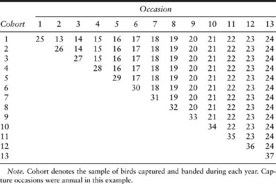
The AIC selection criteria that will be used to compare between models assume that at least one of the models under consideration is an adequate representation of the data (Burnham and Anderson 1998). Therefore, the goodness of fit of the global model should be tested before continuing with model construction. Goodness-of-fit testing by parametric bootstrapping in MARK requires a temporary switch to an alternate parameterization, denoted (S, r), as discussed in chapter 10 of Cooch and White (2001). Fortunately, MARK allows a change of the parameterization scheme mid-analysis. Highlight model (St, ![]() ) in the Results Browser window, select “Change Data Type” from the PIM drop-down menu on the main toolbar, and select the “Dead Recoveries” data type in the window that appears. Now rerun the model with name (St,
) in the Results Browser window, select “Change Data Type” from the PIM drop-down menu on the main toolbar, and select the “Dead Recoveries” data type in the window that appears. Now rerun the model with name (St, ![]() ). Note that the new parameterization does not change the logic behind the model or the way it fits the data, as confirmed by identical results for models (St,
). Note that the new parameterization does not change the logic behind the model or the way it fits the data, as confirmed by identical results for models (St, ![]() ) and (St,
) and (St, ![]() ) in the Results Browser window. Select “Bootstrap GOF” from the Tests drop-down menu on the main toolbar, designate an output file, and run between 500 and 1000 simulations. Once completed, select “View Simulation results” from the Simulations drop-down menu on the main toolbar and open the output file. The simulation results can be sorted according to deviance by clicking the 3rd button from the right in the Browse Database window. Recall from the Results Browser window that the deviance of model (St,
) in the Results Browser window. Select “Bootstrap GOF” from the Tests drop-down menu on the main toolbar, designate an output file, and run between 500 and 1000 simulations. Once completed, select “View Simulation results” from the Simulations drop-down menu on the main toolbar and open the output file. The simulation results can be sorted according to deviance by clicking the 3rd button from the right in the Browse Database window. Recall from the Results Browser window that the deviance of model (St, ![]() ) was 35.9. Comparison of this value to the simulation results reveals that most of the simulations have appreciably higher deviances than the actual model. The data sets from which the simulation deviances were derived were created to fit the selected model and satisfy all assumptions. If the global model were a poor fit to the data, we would expect the deviances of the simulations to be smaller than that of the global model. Because most of the deviances from the simulation data sets exceeded that of the global model, it appears that the global model does indeed adequately fit the data.
) was 35.9. Comparison of this value to the simulation results reveals that most of the simulations have appreciably higher deviances than the actual model. The data sets from which the simulation deviances were derived were created to fit the selected model and satisfy all assumptions. If the global model were a poor fit to the data, we would expect the deviances of the simulations to be smaller than that of the global model. Because most of the deviances from the simulation data sets exceeded that of the global model, it appears that the global model does indeed adequately fit the data.
A reasonable list of restricted models can now be developed for the mallard data. Comparison between these models will reveal which biological effects are supported by the data, thus providing a means of hypothesis testing. Less parameterized models may have higher estimated precision than the global model, but also may show an increased level of bias. AIC and its derivatives provides an objective method for evaluating this trade-off and selecting the best model.
The mallard analysis began with the MARK default model, (St, ft), and the global model (St, ![]() ), which allowed for a banding effect in addition to full time dependence. A logical next step is to investigate the significance of time dependence in each parameter separately by building three additional models—(St, f.), (S., ft), and (S., f.). As before, these models are created through the PIMs. For example, the notation (S., f.) corresponds to a model that restricts both Si and fi to be constant for the duration of the study. Both PIMs for this model should therefore contain the same index value for all rows and columns (recall that PIM columns correspond to study years, as shown in table 9.23).
), which allowed for a banding effect in addition to full time dependence. A logical next step is to investigate the significance of time dependence in each parameter separately by building three additional models—(St, f.), (S., ft), and (S., f.). As before, these models are created through the PIMs. For example, the notation (S., f.) corresponds to a model that restricts both Si and fi to be constant for the duration of the study. Both PIMs for this model should therefore contain the same index value for all rows and columns (recall that PIM columns correspond to study years, as shown in table 9.23).
TABLE 9.23
The MARK parameter information matrices (PIMs) for the constant (homogenous) model (S, f) in the Brownie model of for the mallard band-recovery data

Run models (St, f.), (S., ft), and (S., f.) and compare the output in the Results Browser window, which should include all 5 models considered thus far. Ranking the models by AICc shows, for example, a ΔAICc difference of 29.78 between models (S., ft) and (S., f.), which indicates that the data show strong support for time variation in the reporting rate.
At this point, additional biological information is required to proceed with the analysis. As mentioned at the beginning of the example, Nichols et al. (1982a) recognized a negative density dependence in the natural mortality rate of mallards. The significance of this effect can be investigated by modeling survival as a function of the yearly covariate ducks/pond, for which Williams et al. (2002) provided standardized values. In MARK, the modeling of environmental covariates is accomplished through the Design Matrix. See chapter 7 of Cooch and White (2001) for more discussion of the Design Matrix and linear models. For now, retrieve model (St, ft) and select “Full” from the Design drop-down menu on the main toolbar. The corresponding Design Matrix represents the structure of the linear models underlying the time-dependent model.
The goal of modeling the environmental covariate ducks/pond is to add independent information to the analysis, thereby explaining some of the variation in Si without incurring the penalty in AICc associated with the large number of parameters required for full time dependence. In other words, whereas model (St, ft) models survival as a function of 12 coefficients (B1-B12), an alternate covariate model constrains Si to be a linear function of ducks/pond, i.e.,

where xi is the value of ducks/pond for year i, and β0 and β1 are estimated coefficients. This model can be specified in MARK by deleting columns B3-B12 of the time-dependent Design Matrix and entering each year’s value of the covariate ducks/pond into column B2. The resulting Design Matrix represents the model (Scov, ft) and is shown in table 9.24. Name and run this model.
The Results Browser window now includes all models developed to this point. AICc values indicate that (Scov, ft) is the most useful representation of the mallard data because model (Scov, ft) has an appreciably lower deviance than model (S, ft) and requires only 1 more parameter. It can therefore be concluded that survival rates of the adult female mallards in this study were predicted by population density on spring breeding grounds (as represented by ducks/pond), and that the band reporting rates varied from year to year. Parameter estimates for model (Scov, ft) as output by program MARK are displayed in table 9.25.
TABLE 9.24
The MARK design matrix for the reduced-parameter, Brownie et al. model (Scov, ft) fit to the mallard band-recovery data

TABLE 9.25
Covariate (ducks/pond) and estimates of survival probabilities (Si) and recovery probabilities (fi) for mallard tag-recovery data, using model (Scov, fi)

9.9 Chapter Summary
• Empirical examples of models described in earlier chapters were given.
• The Jolly-Seber model was applied to the European dipper data.
• The Manly-Parr model was applied to the European dipper data.
• Cormack-Jolly-Seber model was applied to the European dipper data. This included illustration of three ways to fit the model using program MARK (PIMs, design matrix, and individual covariate). A general regression approach was also provided that avoided PIM’s and MARK’s design matrix.
• Significant liberties were taken with the dipper data and the Huggins closed-population model was applied. This example included illustration of the likelihood in a spreadsheet program.
• The Test 2 and Test 3 goodness-of-fit procedures (available in program RELEASE) were discussed and illustrated. The parametric bootstrap procedure was also described and illustrated using the dipper data. Overdispersion was estimated based on Test 2 and Test 3.
• The Horvitz-Thompson estimator of population size was applied to the dipper data.
• Significant liberties were again taken with the dipper data, it was modified, and a multistate model was applied.
• An involved example of CJS modeling of polar bears in the Southern Beaufort Sea was given.
• An involved example of the Brownie tag-return model applied to mallard data was given.

Figure 9.5. A poncho-marked and leg-banded sharp-tailed grouse (Tympanuchus phasianellus) ready for release near Decker, Montana, spring 1977. (Photo by Steven C. Amstrup)