6.1 Parameter Selection with Preprocessing

Now let’s say we want to find better parameters for SVC using GridSearchCV, as discussed in Chapter 5. How should we go about doing this? A naive approach might look like this:

In[3]:

from sklearn.model_selection import GridSearchCV
# for illustration purposes only, don't use this code!
param_grid = {'C': [0.001, 0.01, 0.1, 1, 10, 100],
              'gamma': [0.001, 0.01, 0.1, 1, 10, 100]}
grid = GridSearchCV(SVC(), param_grid=param_grid, cv=5)
grid.fit(X_train_scaled, y_train)
print("Best cross-validation accuracy: {:.2f}".format(grid.best_score_))
print("Best parameters: ", grid.best_params_)
print("Test set accuracy: {:.2f}".format(grid.score(X_test_scaled, y_test)))

Out[3]:

Best cross-validation accuracy: 0.98
Best parameters:  {'gamma': 1, 'C': 1}
Test set accuracy: 0.97

Here, we ran the grid search over the parameters of SVC using the scaled data. However, there is a subtle catch in what we just did. When scaling the data, we used all the data in the training set to compute the minimum and maximum of the data. We then use the scaled training data to run our grid search using cross-validation. For each split in the cross-validation, some part of the original training set will be declared the training part of the split, and some the test part of the split. The test part is used to measure the performance of a model trained on the training part when applied to new data. However, we already used the information contained in the test part of the split, when scaling the data. Remember that the test part in each split in the cross-validation is part of the training set, and we used the information from the entire training set to find the right scaling of the data. This is fundamentally different from how new data looks to the model. If we observe new data (say, in form of our test set), this data will not have been used to scale the training data, and it might have a different minimum and maximum than the training data. The following example (Figure 6-1) shows how the data processing during cross-validation and the final evaluation differ:

In[4]:

mglearn.plots.plot_improper_processing()

Figure 6-1. Data usage when preprocessing outside the cross-validation loop

So, the splits in the cross-validation no longer correctly mirror how new data will look to the modeling process. We already leaked information from these parts of the data into our modeling process. This will lead to overly optimistic results during cross-validation, and possibly the selection of suboptimal parameters.

To get around this problem, the splitting of the dataset during cross-validation should be done before doing any preprocessing. Any process that extracts knowledge from the dataset should only ever be learned from the training portion of the dataset, and therefore be contained inside the cross-validation loop.

To achieve this in scikit-learn with the cross_val_score function and the GridSearchCV function, we can use the Pipeline class. The Pipeline class is a class that allows “gluing” together multiple processing steps into a single scikit-learn estimator. The Pipeline class itself has fit, predict, and score methods and behaves just like any other model in scikit-learn. The most common use case of the Pipeline class is in chaining preprocessing steps (like scaling of the data) together with a supervised model like a classifier.

6.2 Building Pipelines

Let’s look at how we can use the Pipeline class to express the workflow for training an SVM after scaling the data with MinMaxScaler (for now without the grid search). First, we build a pipeline object by providing it with a list of steps. Each step is a tuple containing a name (any string of your choosing¹) and an instance of an estimator:

In[5]:

from sklearn.pipeline import Pipeline
pipe = Pipeline([("scaler", MinMaxScaler()), ("svm", SVC())])

Here, we created two steps: the first, called "scaler", is an instance of MinMaxScaler, and the second, called "svm", is an instance of SVC. Now, we can fit the pipeline, like any other scikit-learn estimator:

In[6]:

pipe.fit(X_train, y_train)

Here, pipe.fit first calls fit on the first step (the scaler), then transforms the training data using the scaler, and finally fits the SVM with the scaled data. To evaluate on the test data, we simply call pipe.score:

In[7]:

print("Test score: {:.2f}".format(pipe.score(X_test, y_test)))

Out[7]:

Test score: 0.95

Calling the score method on the pipeline first transforms the test data using the scaler, and then calls the score method on the SVM using the scaled test data. As you can see, the result is identical to the one we got from the code at the beginning of the chapter, when doing the transformations by hand. Using the pipeline, we reduced the code needed for our “preprocessing + classification” process. The main benefit of using the pipeline, however, is that we can now use this single estimator in cross_val_score or GridSearchCV.

6.3 Using Pipelines in Grid Searches

Using a pipeline in a grid search works the same way as using any other estimator. We define a parameter grid to search over, and construct a GridSearchCV from the pipeline and the parameter grid. When specifying the parameter grid, there is a slight change, though. We need to specify for each parameter which step of the pipeline it belongs to. Both parameters that we want to adjust, C and gamma, are parameters of SVC, the second step. We gave this step the name "svm". The syntax to define a parameter grid for a pipeline is to specify for each parameter the step name, followed by __ (a double underscore), followed by the parameter name. To search over the C parameter of SVC we therefore have to use "svm__C" as the key in the parameter grid dictionary, and similarly for gamma:

In[8]:

param_grid = {'svm__C': [0.001, 0.01, 0.1, 1, 10, 100],
              'svm__gamma': [0.001, 0.01, 0.1, 1, 10, 100]}

With this parameter grid we can use GridSearchCV as usual:

In[9]:

grid = GridSearchCV(pipe, param_grid=param_grid, cv=5)
grid.fit(X_train, y_train)
print("Best cross-validation accuracy: {:.2f}".format(grid.best_score_))
print("Test set score: {:.2f}".format(grid.score(X_test, y_test)))
print("Best parameters: {}".format(grid.best_params_))

Out[9]:

Best cross-validation accuracy: 0.98
Test set score: 0.97
Best parameters: {'svm__C': 1, 'svm__gamma': 1}

In contrast to the grid search we did before, now for each split in the cross-validation, the MinMaxScaler is refit with only the training splits and no information is leaked from the test split into the parameter search. Compare this (Figure 6-2) with Figure 6-1 earlier in this chapter:

In[10]:

mglearn.plots.plot_proper_processing()

Figure 6-2. Data usage when preprocessing inside the cross-validation loop with a pipeline

The impact of leaking information in the cross-validation varies depending on the nature of the preprocessing step. Estimating the scale of the data using the test fold usually doesn’t have a terrible impact, while using the test fold in feature extraction and feature selection can lead to substantial differences in outcomes.

6.4 The General Pipeline Interface

The Pipeline class is not restricted to preprocessing and classification, but can in fact join any number of estimators together. For example, you could build a pipeline containing feature extraction, feature selection, scaling, and classification, for a total of four steps. Similarly, the last step could be regression or clustering instead of classification.

The only requirement for estimators in a pipeline is that all but the last step need to have a transform method, so they can produce a new representation of the data that can be used in the next step.

Internally, during the call to Pipeline.fit, the pipeline calls fit and then transform on each step in turn,² with the input given by the output of the transform method of the previous step. For the last step in the pipeline, just fit is called.

Brushing over some finer details, this is implemented as follows. Remember that pipeline.steps is a list of tuples, so pipeline.steps[0][1] is the first estimator, pipeline.steps[1][1] is the second estimator, and so on:

In[15]:

def fit(self, X, y):
    X_transformed = X
    for name, estimator in self.steps[:-1]:
        # iterate over all but the final step
        # fit and transform the data
        X_transformed = estimator.fit_transform(X_transformed, y)
    # fit the last step
    self.steps[-1][1].fit(X_transformed, y)
    return self

When predicting using Pipeline, we similarly transform the data using all but the last step, and then call predict on the last step:

In[16]:

def predict(self, X):
    X_transformed = X
    for step in self.steps[:-1]:
        # iterate over all but the final step
        # transform the data
        X_transformed = step[1].transform(X_transformed)
    # predict using the last step
    return self.steps[-1][1].predict(X_transformed)

The process is illustrated in Figure 6-3 for two transformers, T1 and T2, and a classifier (called Classifier).

Figure 6-3. Overview of the pipeline training and prediction process

The pipeline is actually even more general than this. There is no requirement for the last step in a pipeline to have a predict function, and we could create a pipeline just containing, for example, a scaler and PCA. Then, because the last step (PCA) has a transform method, we could call transform on the pipeline to get the output of PCA.transform applied to the data that was processed by the previous step. The last step of a pipeline is only required to have a fit method.

from sklearn.pipeline import make_pipeline
# standard syntax
pipe_long = Pipeline([("scaler", MinMaxScaler()), ("svm", SVC(C=100))])
# abbreviated syntax
pipe_short = make_pipeline(MinMaxScaler(), SVC(C=100))

print("Pipeline steps:
{}".format(pipe_short.steps))

Pipeline steps:
[('minmaxscaler', MinMaxScaler(copy=True, feature_range=(0, 1))),
 ('svc', SVC(C=100, cache_size=200, class_weight=None, coef0=0.0,
	     decision_function_shape='ovr', degree=3, gamma='auto',
             kernel='rbf', max_iter=-1, probability=False,
             random_state=None, shrinking=True, tol=0.001,
             verbose=False))]

from sklearn.preprocessing import StandardScaler
from sklearn.decomposition import PCA

pipe = make_pipeline(StandardScaler(), PCA(n_components=2), StandardScaler())
print("Pipeline steps:
{}".format(pipe.steps))

Pipeline steps:
[('standardscaler-1', StandardScaler(copy=True, with_mean=True, with_std=True)),
 ('pca', PCA(copy=True, iterated_power='auto', n_components=2, random_state=None,
             svd_solver='auto', tol=0.0, whiten=False)),
 ('standardscaler-2', StandardScaler(copy=True, with_mean=True, with_std=True))]

# fit the pipeline defined before to the cancer dataset
pipe.fit(cancer.data)
# extract the first two principal components from the "pca" step
components = pipe.named_steps["pca"].components_
print("components.shape: {}".format(components.shape))

components.shape: (2, 30)

from sklearn.linear_model import LogisticRegression

pipe = make_pipeline(StandardScaler(), LogisticRegression())

param_grid = {'logisticregression__C': [0.01, 0.1, 1, 10, 100]}

X_train, X_test, y_train, y_test = train_test_split(
    cancer.data, cancer.target, random_state=4)
grid = GridSearchCV(pipe, param_grid, cv=5)
grid.fit(X_train, y_train)

print("Best estimator:
{}".format(grid.best_estimator_))

Best estimator:
Pipeline(memory=None, steps=[
    ('standardscaler', StandardScaler(copy=True, with_mean=True, with_std=True)),
    ('logisticregression', LogisticRegression(C=0.1, class_weight=None,
    dual=False, fit_intercept=True, intercept_scaling=1, max_iter=100,
    multi_class='warn', n_jobs=None, penalty='l2', random_state=None,
    solver='warn', tol=0.0001, verbose=0, warm_start=False))])

print("Logistic regression step:
{}".format(
      grid.best_estimator_.named_steps["logisticregression"]))

Logistic regression step:
LogisticRegression(C=0.1, class_weight=None, dual=False, fit_intercept=True,
                  intercept_scaling=1, max_iter=100, multi_class='warn',
                  n_jobs=None, penalty='l2', random_state=None, solver='warn',
                  tol=0.0001, verbose=0, warm_start=False)

print("Logistic regression coefficients:
{}".format(
      grid.best_estimator_.named_steps["logisticregression"].coef_))

Logistic regression coefficients:
[[-0.389 -0.375 -0.376 -0.396 -0.115  0.017 -0.355 -0.39  -0.058  0.209
  -0.495 -0.004 -0.371 -0.383 -0.045  0.198  0.004 -0.049  0.21   0.224
  -0.547 -0.525 -0.499 -0.515 -0.393 -0.123 -0.388 -0.417 -0.325 -0.139]]

6.5 Grid-Searching Preprocessing Steps and Model Parameters

Using pipelines, we can encapsulate all the processing steps in our machine learning workflow in a single scikit-learn estimator. Another benefit of doing this is that we can now adjust the parameters of the preprocessing using the outcome of a supervised task like regression or classification. In previous chapters, we used polynomial features on the boston dataset before applying the ridge regressor. Let’s model that using a pipeline instead. The pipeline contains three steps—scaling the data, computing polynomial features, and ridge regression:

In[27]:

from sklearn.datasets import load_boston
boston = load_boston()
X_train, X_test, y_train, y_test = train_test_split(boston.data, boston.target,
                                                    random_state=0)

from sklearn.preprocessing import PolynomialFeatures
pipe = make_pipeline(
    StandardScaler(),
    PolynomialFeatures(),
    Ridge())

How do we know which degrees of polynomials to choose, or whether to choose any polynomials or interactions at all? Ideally we want to select the degree parameter based on the outcome of the classification. Using our pipeline, we can search over the degree parameter together with the parameter alpha of Ridge. To do this, we define a param_grid that contains both, appropriately prefixed by the step names:

In[28]:

param_grid = {'polynomialfeatures__degree': [1, 2, 3],
              'ridge__alpha': [0.001, 0.01, 0.1, 1, 10, 100]}

Now we can run our grid search again:

In[29]:

grid = GridSearchCV(pipe, param_grid=param_grid, cv=5, n_jobs=-1)
grid.fit(X_train, y_train)

We can visualize the outcome of the cross-validation using a heat map (Figure 6-4), as we did in Chapter 5:

In[30]:

plt.matshow(grid.cv_results_['mean_test_score'].reshape(3, -1),
            vmin=0, cmap="viridis")
plt.xlabel("ridge__alpha")
plt.ylabel("polynomialfeatures__degree")
plt.xticks(range(len(param_grid['ridge__alpha'])), param_grid['ridge__alpha'])
plt.yticks(range(len(param_grid['polynomialfeatures__degree'])),
           param_grid['polynomialfeatures__degree'])

plt.colorbar()

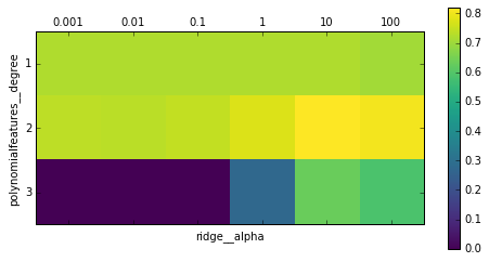
Figure 6-4. Heat map of mean cross-validation score as a function of the degree of the polynomial features and alpha parameter of Ridge

Looking at the results produced by the cross-validation, we can see that using polynomials of degree two helps, but that degree-three polynomials are much worse than either degree one or two. This is reflected in the best parameters that were found:

In[31]:

print("Best parameters: {}".format(grid.best_params_))

Out[31]:

Best parameters: {'polynomialfeatures__degree': 2, 'ridge__alpha': 10}

Which lead to the following score:

In[32]:

print("Test-set score: {:.2f}".format(grid.score(X_test, y_test)))

Out[32]:

Test-set score: 0.77

Let’s run a grid search without polynomial features for comparison:

In[33]:

param_grid = {'ridge__alpha': [0.001, 0.01, 0.1, 1, 10, 100]}
pipe = make_pipeline(StandardScaler(), Ridge())
grid = GridSearchCV(pipe, param_grid, cv=5)
grid.fit(X_train, y_train)
print("Score without poly features: {:.2f}".format(grid.score(X_test, y_test)))

Out[33]:

Score without poly features: 0.63

As we would expect looking at the grid search results visualized in Figure 6-4, using no polynomial features leads to decidedly worse results.

Searching over preprocessing parameters together with model parameters is a very powerful strategy. However, keep in mind that GridSearchCV tries all possible combinations of the specified parameters. Therefore, adding more parameters to your grid exponentially increases the number of models that need to be built.

6.6 Grid-Searching Which Model To Use

You can even go further in combining GridSearchCV and Pipeline: it is also possible to search over the actual steps being performed in the pipeline (say whether to use StandardScaler or MinMaxScaler). This leads to an even bigger search space and should be considered carefully. Trying all possible solutions is usually not a viable machine learning strategy. However, here is an example comparing a RandomForestClassifier and an SVC on the iris dataset. We know that the SVC might need the data to be scaled, so we also search over whether to use StandardScaler or no preprocessing. For the RandomForestClassifier, we know that no preprocessing is necessary. We start by defining the pipeline. Here, we explicitly name the steps. We want two steps, one for the preprocessing and then a classifier. We can instantiate this using SVC and StandardScaler:

In[34]:

pipe = Pipeline([('preprocessing', StandardScaler()), ('classifier', SVC())])

Now we can define the parameter_grid to search over. We want the classifier to be either RandomForestClassifier or SVC. Because they have different parameters to tune, and need different preprocessing, we can make use of the list of search grids we discussed in “Search over spaces that are not grids”. To assign an estimator to a step, we use the name of the step as the parameter name. When we wanted to skip a step in the pipeline (for example, because we don’t need preprocessing for the RandomForest), we can set that step to None:

In[35]:

from sklearn.ensemble import RandomForestClassifier

param_grid = [
    {'classifier': [SVC()], 'preprocessing': [StandardScaler(), None],
     'classifier__gamma': [0.001, 0.01, 0.1, 1, 10, 100],
     'classifier__C': [0.001, 0.01, 0.1, 1, 10, 100]},
    {'classifier': [RandomForestClassifier(n_estimators=100)],
     'preprocessing': [None], 'classifier__max_features': [1, 2, 3]}]

Now we can instantiate and run the grid search as usual, here on the cancer dataset:

In[36]:

X_train, X_test, y_train, y_test = train_test_split(
    cancer.data, cancer.target, random_state=0)

grid = GridSearchCV(pipe, param_grid, cv=5)
grid.fit(X_train, y_train)

print("Best params:
{}
".format(grid.best_params_))
print("Best cross-validation score: {:.2f}".format(grid.best_score_))
print("Test-set score: {:.2f}".format(grid.score(X_test, y_test)))

Out[36]:

Best params:
{'classifier':
 SVC(C=10, cache_size=200, class_weight=None, coef0=0.0,
     decision_function_shape='ovr', degree=3, gamma=0.01, kernel='rbf',
     max_iter=-1, probability=False, random_state=None, shrinking=True,
     tol=0.001, verbose=False),
 'preprocessing':
 StandardScaler(copy=True, with_mean=True, with_std=True),
 'classifier__C': 10, 'classifier__gamma': 0.01}

Best cross-validation score: 0.99
Test-set score: 0.98

The outcome of the grid search is that SVC with StandardScaler preprocessing, C=10, and gamma=0.01 gave the best result.

pipe = Pipeline([('preprocessing', StandardScaler()), ('classifier', SVC())],
                memory="cache_folder")

6.7 Summary and Outlook

In this chapter we introduced the Pipeline class, a general-purpose tool to chain together multiple processing steps in a machine learning workflow. Real-world applications of machine learning rarely involve an isolated use of a model, and instead are a sequence of processing steps. Using pipelines allows us to encapsulate multiple steps into a single Python object that adheres to the familiar scikit-learn interface of fit, predict, and transform. In particular when doing model evaluation using cross-validation and parameter selection using grid search, using the Pipeline class to capture all the processing steps is essential for proper evaluation. The Pipeline class also allows writing more succinct code, and reduces the likelihood of mistakes that can happen when building processing chains without the pipeline class (like forgetting to apply all transformers on the test set, or not applying them in the right order). Choosing the right combination of feature extraction, preprocessing, and models is somewhat of an art, and often requires some trial and error. However, using pipelines, this “trying out” of many different processing steps is quite simple. When experimenting, be careful not to overcomplicate your processes, and make sure to evaluate whether every component you are including in your model is necessary.

With this chapter, we have completed our survey of general-purpose tools and algorithms provided by scikit-learn. You now possess all the required skills and know the necessary mechanisms to apply machine learning in practice. In the next chapter, we will dive in more detail into one particular type of data that is commonly seen in practice, and that requires some special expertise to handle correctly: text data.