Chapter 6. Data Parallelism
I’ve previously made a lot of references to the idea that it’s easier to write parallel code in Java 8. This is because we can use lambda expressions in combination with the streams library, introduced in Chapter 3, to say what we want our program to do, regardless of whether it’s sequential or parallel. I know that sounds a lot like what you’ve been doing in Java for years, but there’s a difference between saying what you want to compute and saying how to compute it.
The big shift between external and internal iteration (also discussed in Chapter 3) did make it easier to write simple and clean code, but here’s the other big benefit: now we don’t have to manually control the iteration. It doesn’t need to be performed sequentially. We express the what and, by changing a single method call, we can get a library to figure out the how.
The changes to your code are surprisingly unobtrusive, so the majority of this chapter won’t be talking about how your code changes. Instead, I’ll explain why you might want to go parallel and when you’ll get performance improvements. It’s also worth noting that this chapter isn’t a general text on performance in Java; we’ll just be looking at the easy wins provided in Java 8.
Parallelism Versus Concurrency
After a quick scan over the table of contents of this book, you might have noticed this chapter with the word parallelism in the title and also Chapter 9, which has concurrency in the title. Don’t worry—I haven’t repeated the same material in an attempt to justify charging you more for this book! Concurrency and parallelism are different things that can be leveraged to achieve different aims.
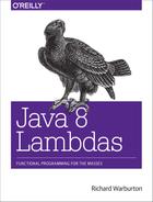
Concurrency arises when two tasks are making progress at overlapping time periods. Parallelism arises when two tasks are happening at literally the same time, such as on a multicore CPU. If a program is undertaking two tasks and they are being given small slices of a single CPU core’s time, then it is exhibiting concurrency but not parallelism. This difference is shown in Figure 6-1.
The goal of parallelism is to reduce the runtime of a specific task by breaking it down into smaller components and performing them in parallel. This doesn’t mean that you won’t do as much work as you would if you were running them sequentially—you are just getting more horses to pull the same cart for a shorter time period. In fact, it’s usually the case that running a task in parallel requires more work to be done by the CPU than running it sequentially would.
In this chapter, we’re looking at a very specific form of parallelism called data parallelism. In data parallelism, we achieve parallelism by splitting up the data to be operated on and assigning a single processing unit to each chunk of data. If we’re to extend our horses-pulling-carts analogy, it would be like taking half of the goods inside our cart and putting them into another cart for another horse to pull, with both horses taking an identical route to the destination.
Data parallelism works really well when you want to perform the same operation on a lot of data. The problem needs be decomposed in a way that will work on subsections of the data, and then the answers from each subsection can be composed at the end.
Data parallelism is often contrasted with task parallelism, in which each individual thread of execution can be doing a totally different task. Probably the most commonly encountered task parallelism is a Java EE application container. Each thread not only can be dealing with processing a different user, but also could be performing different tasks for a user, such as logging in or adding an item to a shopping cart.
Why Is Parallelism Important?
Historically, we could all rely on the clock frequency of a CPU getting faster over time. Intel’s 8086 processor, introduced in 1979, started at a 5 MHz clock rate, and by the time the Pentium chip was introduced in 1993 speeds had reached 60 MHz. Improved sequential performance continued through the early 2000s.
Over the last decade, however, mainstream chip manufacturers have been moving increasingly toward heavily multicore processors. At the time of writing, it’s not uncommon for servers to be shipping with 32 or 64 cores spread over several physical processing units. This trend shows no sign of abating soon.
This influences the design of software. Instead of being able to rely on improved CPU clock speeds to increase the computational capacity of existing code, we need to be able to take advantage of modern CPU architectures. The only way to do this is by writing parallel programs.
I appreciate you’ve probably heard this message before. In fact, it’s one that’s been blasted out by many conference speakers, book authors, and consultants over the years. The implications of Amdahl’s Law were what really made me take note of the importance of parallelism.
Amdahl’s Law is a simple rule that predicts the theoretical maximum speedup of a program on a machine with multiple cores. If we take a program that is entirely serial and parallelize only half of it, then the maximum speedup possible, regardless of how many cores we throw at the problem, is 2×. Given a large number of cores—and we’re already into that territory—the execution time of a problem is going to be dominated by the serial part of that problem.
When you start to think of performance in these terms, optimizing any job that is bound by computational work rapidly becomes a matter of ensuring that it effectively utilizes the available hardware. Of course, not every job is bound by computational work, but in this chapter we’ll be focusing on that kind of problem.
Parallel Stream Operations
Making an operation execute in parallel using the streams library is a
matter of changing a single method call. If you already have a Stream object,
then you can call its parallel method in order to make it parallel. If
you’re creating a Stream from a Collection, you can call the
parallelStream method in order to create a parallel stream from the get-go.
Let’s look at a simple example in order to make things concrete. Example 6-1 calculates the total length of a sequence of albums. It transforms each album into its component tracks, then gets into the length of each track, and then sums them.
publicintserialArraySum(){returnalbums.stream().flatMap(Album::getTracks).mapToInt(Track::getLength).sum();}
We go parallel by making the call to parallelStream, as shown in Example 6-2; all the rest of the code is identical. Going parallel just works.
publicintparallelArraySum(){returnalbums.parallelStream().flatMap(Album::getTracks).mapToInt(Track::getLength).sum();}
I know the immediate instinct upon hearing this is to go out and
replace every call to stream with a call to parallelStream because it’s so
easy. Hold your horses for a moment! Obviously it’s important to make good
use of parallelism in order to get the most from your hardware, but the kind of
data parallelism we get from the streams library is only one form.
The question we really want to ask ourselves is whether it’s faster to run our
Stream-based code sequentially or in parallel, and that’s not a question
with an easy answer. If we look back at the previous example, where we
figure out the total running time of a list of albums, depending upon the
circumstances we can make the sequential or parallel versions faster.
When benchmarking the code in Examples 6-1 and 6-2 on a 4-core machine with 10 albums, the sequential code was 8× faster. Upon expanding the number of albums to 100, they were both equally fast, and by the time we hit 10,000 albums, the parallel code was 2.5× faster.
Note
Any specific benchmark figures in this chapter are listed only to make a point. If you try to replicate these results on your hardware, you may get drastically different outcomes.
The size of the input stream isn’t the only factor to think about when deciding whether there’s a parallel speedup. It’s possible to get varying performance numbers based upon how you wrote your code and how many cores are available. We’ll look at this in a bit more detail in Performance, but first let’s look at a more complex example.
Simulations
The kinds of problems that parallel stream libraries excel at are those that involve simple operations processing a lot of data, such as simulations. In this section, we’ll be building a simple simulation to understand dice throws, but the same ideas and approach can be used on larger and more realistic problems.
The kind of simulation we’ll be looking at here is a Monte Carlo simulation. Monte Carlo simulations work by running the same simulation many times over with different random seeds on every run. The results of each run are recorded and aggregated in order to build up a comprehensive simulation. They have many uses in engineering, finance, and scientific computing.
If we throw a fair die twice and add up the number of dots on the winning side, we’ll get a number between 2 and 12. This must be at least 2 because the fewest number of dots on each side is 1 and there are two dice. The maximum score is 12, as the highest number you can score on each die is 6. We want to try and figure out what the probability of each number between 2 and 12 is.
One approach to solving this problem is to add up all the different combinations of dice rolls that can get us each value. For example, the only way we can get 2 is by rolling 1 and then 1 again. There are 36 different possible combinations, so the probability of the two sides adding up to 2 is 1 in 36, or 1/36.
Another way of working it out is to simulate rolling two dice using random numbers between 1 and 6, adding up the number of times that each result was picked, and dividing by the number of rolls. This is actually a really simple Monte Carlo simulation. The more times we simulate rolling the dice, the more closely we approximate the actual result—so we really want to do it a lot.
Example 6-3 shows how we can implement the Monte Carlo approach using the streams library. N represents the number of simulations we’ll be running, and at ![]() we use the
we use the IntStream range function to create a stream of size N. At ![]() we call the
we call the parallel method in order to use the parallel version of the streams framework. The twoDiceThrows function simulates throwing two dice and returns the sum of their results. We use the mapToObj method in ![]() in order to use this function on our data stream.
in order to use this function on our data stream.
At ![]() we have a
we have a Stream of all the simulation results we need to combine. We use the groupingBy collector, introduced in the previous chapter, in order to aggregate all results that are equal. I said we were going to count the number of times each number occured and divide by N. In the streams framework, it’s actually easier to map numbers to 1/N and add them, which is exactly the same. This is accomplished in ![]() through the
through the summingDouble function. The Map<Integer, Double> that gets returned at the end maps each sum of sides thrown to its probability.
I’ll admit it’s not totally trivial code, but implementing a parallel Monte Carlo simulation in five lines of code is pretty neat. Importantly, because the more simulations we run, the more closey we approximate the real answer, we’ve got a real incentive to run a lot of simulations. This is also a good use for parallelism as it’s an implementation that gets good parallel speedup.
I won’t go through the implementation details, but for comparison Example 6-4 lists the same parallel Monte Carlo simulation implemented by hand. The majority of the code implementation deals with spawning, scheduling, and awaiting the completion of jobs within a thread pool. None of these issues needs to be directly addressed when using the parallel streams library.
publicclassManualDiceRolls{privatestaticfinalintN=100000000;privatefinaldoublefraction;privatefinalMap<Integer,Double>results;privatefinalintnumberOfThreads;privatefinalExecutorServiceexecutor;privatefinalintworkPerThread;publicstaticvoidmain(String[]args){ManualDiceRollsroles=newManualDiceRolls();roles.simulateDiceRoles();}publicManualDiceRolls(){fraction=1.0/N;results=newConcurrentHashMap<>();numberOfThreads=Runtime.getRuntime().availableProcessors();executor=Executors.newFixedThreadPool(numberOfThreads);workPerThread=N/numberOfThreads;}publicvoidsimulateDiceRoles(){List<Future<?>>futures=submitJobs();awaitCompletion(futures);printResults();}privatevoidprintResults(){results.entrySet().forEach(System.out::println);}privateList<Future<?>>submitJobs(){List<Future<?>>futures=newArrayList<>();for(inti=0;i<numberOfThreads;i++){futures.add(executor.submit(makeJob()));}returnfutures;}privateRunnablemakeJob(){return()->{ThreadLocalRandomrandom=ThreadLocalRandom.current();for(inti=0;i<workPerThread;i++){intentry=twoDiceThrows(random);accumulateResult(entry);}};}privatevoidaccumulateResult(intentry){results.compute(entry,(key,previous)->previous==null?fraction:previous+fraction);}privateinttwoDiceThrows(ThreadLocalRandomrandom){intfirstThrow=random.nextInt(1,7);intsecondThrow=random.nextInt(1,7);returnfirstThrow+secondThrow;}privatevoidawaitCompletion(List<Future<?>>futures){futures.forEach((future)->{try{future.get();}catch(InterruptedException|ExecutionExceptione){e.printStackTrace();}});executor.shutdown();}}
Caveats
I said earlier that using parallel streams “just works,” but that’s being a little cheeky. You can run existing code in parallel with little modification, but only if you’ve written idiomatic code. There are a few rules and restrictions that need to be obeyed in order to make optimal use of the parallel streams framework.
Previously, when calling reduce our initial element could be any value, but
for this operation to work correctly in parallel, it needs to be the identity
value of the combining function. The identity value leaves all other
elements the same when reduced with them. For example, if we’re summing
elements with our reduce operation, the combining function is (acc,
element) -> acc + element. The initial element must be 0, because any
number x added to 0 returns x.
The other caveat specific to reduce is that the combining function must be
associative. This means that the order in which the combining function is
applied doesn’t matter as long the values of the sequence aren’t changed.
Confused? Don’t worry! Take a look at Example 6-5, which shows how
we can rearrange the order in which we apply + and * to a sequence of
values and get the same result.
One thing to avoid is trying to hold locks. The streams framework deals with any necessary synchronization itself, so there’s no need to lock your data structures. If you do try to hold locks on any data structure that the streams library is using, such as the source collection of an operation, you’re likely to run into trouble.
I explained earlier that you could convert any existing Stream to be a
parallel stream using the parallel method call. If you’ve been looking at
the API itself while reading the book, you may have noticed a
sequential method as well. When a stream pipeline is evaluated, there is no
mixed mode: the orientation is either parallel or sequential. If a pipeline has
calls to both parallel and sequential, the last call wins.
Performance
I briefly mentioned before that there were a number of factors that influenced whether parallel streams were faster or slower than sequential streams; let’s take a look at those factors now. Understanding what works well and what doesn’t will help you to make an informed decision about how and when to use parallel streams. There are five important factors that influence parallel streams performance that we’ll be looking at:
- Data size
- There is a difference in the efficiency of the parallel speedup due to the size of the input data. There’s an overhead to decomposing the problem to be executed in parallel and merging the results. This makes it worth doing only when there’s enough data that execution of a streams pipeline takes a while. We explored this back in Parallel Stream Operations.
- Source data structure
- Each pipeline of operations operates on some initial data source; this is usually a collection. It’s easier to split out subsections of different data sources, and this cost affects how much parallel speedup you can get when executing your pipeline.
- Packing
- Primitives are faster to operate on than boxed values.
- Number of cores
- The extreme case here is that you have only a single core available to operate upon, so it’s not worth going parallel. Obviously, the more cores you have access to, the greater your potential speedup is. In practice, what counts isn’t just the number of cores allocated to your machine; it’s the number of cores that are available for your machine to use at runtime. This means factors such as other processes executing simultaneously or thread affinity (forcing threads to execute on certain cores or CPUs) will affect performance.
- Cost per element
- Like data size, this is part of the battle between time spent executing in parallel and overhead of decomposition and merging. The more time spent operating on each element in the stream, the better performance you’ll get from going parallel.
When using the parallel streams framework, it can be helpful to understand how problems are decomposed and merged. This gives us a good insight into what is going on under the hood without having to understand all the details of the framework.
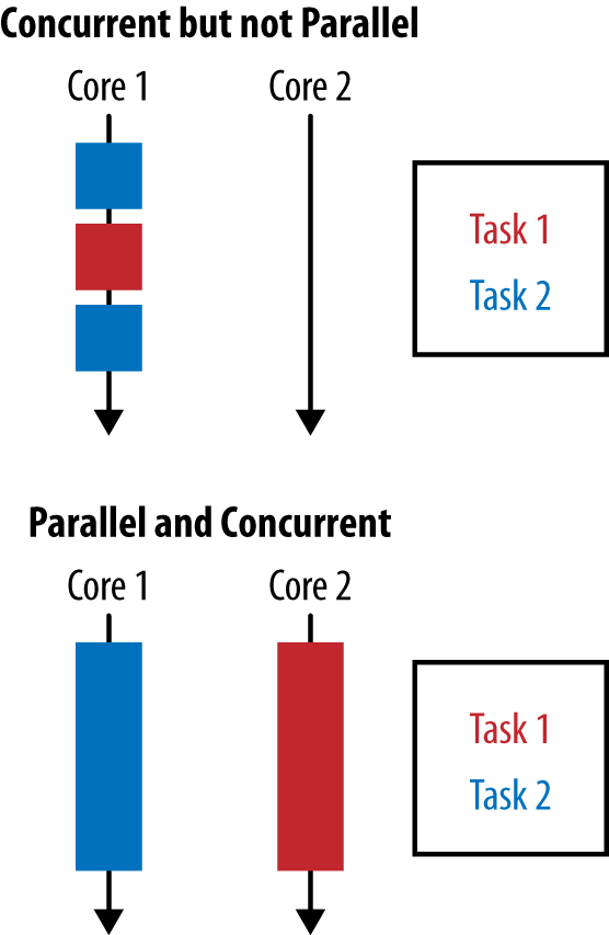
Let’s take a look at how a concrete example is decomposed and merged. Example 6-6 shows some code that performs parallel integer addition.
privateintaddIntegers(List<Integer>values){returnvalues.parallelStream().mapToInt(i->i).sum();}
Under the hood, parallel streams back onto the fork/join framework. The fork stage recursively splits up a problem. Then each chunk is operated upon in parallel. Finally, the join stage merges the results back together.
Figure 6-2 shows how this might apply to Example 6-6.
Let’s assume that the streams framework is splitting up our work to operate in parallel on a four-core machine:
- Our data source is decomposed into four chunks of elements.
-
We perform leaf computation work in parallel on each thread in
Example 6-6. This involves mapping each
Integerto anintand also summing a quarter of the values in each thread. Ideally, we want to spend as much of our time as possible in leaf computation work because it’s the perfect case for parallelism. -
We merge the results. In Example 6-6 this is just a
sumoperation, but it might involve any kind ofreduce,collect, or terminal operation.
Given the way problems are decomposed, the nature of the initial source is extremely important in influencing the performance of this decomposition. Intuitively, the ease with which we can repeatedly split a data structure in half corresponds to how fast it can be operated upon. Splitting in half also means that the values to be operated upon need to split equally.
We can split up common data sources from the core library into three main groups by performance characteristics:
- The good
-
An
ArrayList, an array, or theIntStream.rangeconstructor. These data sources all support random access, which means they can be split up arbitrarily with ease. - The okay
-
The
HashSetandTreeSet. You can’t easily decompose these with perfect amounts of balance, but most of the time it’s possible to do so. - The bad
-
Some data structures just don’t split well; for example, they may take O(N) time to decompose. Examples here include a
LinkedList, which is computationally hard to split in half. Also,Streams.iterateandBufferedReader.lineshave unknown length at the beginning, so it’s pretty hard to estimate when to split these sources.
The influence of the initial data structure can be huge. To take an extreme
example, benchmarking a parallel sum over 10,000 integers revealed an
ArrayList to be 10 times faster than a LinkedList. This isn’t to say that
your business logic will exhibit the same performance characteristics, but it
does demonstrate how influential these things can be. It’s also far more likely
that data structures such as a LinkedList that have poor decompositions
will also be slower when run in parallel.
Ideally, once the streams framework has decomposed the problem into smaller chunks, we’ll be able to operate on each chunk in its own thread, with no further communication or contention between threads. Unfortunately, reality can get the way of the ideal at times!
When we’re talking about the kinds of operations in our stream pipeline that let us operate on chunks individually, we can differentiate between two types of stream operations: stateless and stateful. Stateless operations need to maintain no concept of state over the whole operation; stateful operations have the overhead and constraint of maintaining state.
If you can get away with using stateless operations, then you will get better
parallel performance. Examples of stateless operations include map, filter,
and flatMap; sorted, distinct, and limit are stateful.
Parallel Array Operations
Java 8 includes a couple of other parallel array operations that utilize lambda expressions outside of the streams framework. Like the operations on the streams framework, these are data parallel operations. Let’s look at how we can use these operations to solve problems that are hard to do in the streams framework.
These operations are all located on the utility class Arrays, which also contains
a bunch of other useful array-related functionality from previous Java versions.
There is a summary in Table 6-1.
| Name | Operation |
| Calculates running totals of the values of an array given an arbitrary function |
| Updates the values in an array using a lambda expression |
| Sorts elements in parallel |
You may have written code similar to Example 6-7 before, where you initialize an
array using a for loop. In this case, we initialize every element to its index in the array.
publicstaticdouble[]imperativeInitilize(intsize){double[]values=newdouble[size];for(inti=0;i<values.length;i++){values[i]=i;}returnvalues;}
We can use the parallelSetAll method in order to do this easily in
parallel. An example of this code is shown in Example 6-8. We
provide an array to operate on and a lambda expression, which calculates the
value given the index. In our example they are the same value. One thing to
note about these methods is that they alter the array that is
passed into the operation, rather than creating a new copy.
publicstaticdouble[]parallelInitialize(intsize){double[]values=newdouble[size];Arrays.parallelSetAll(values,i->i);returnvalues;}
The parallelPrefix operation, on the other hand, is much more useful for
performing accumulation-type calculations over time series of data. It
mutates an array, replacing each element with the sum of that element and its predecessors. I use the term “sum” loosely—it doesn’t need to be
addition; it could be any BinaryOperator.
An example operation that can be calculated by prefix sums is a simple moving average. This takes a rolling window over a time series and produces an average for each instance of that window. For example, if our series of input data is 0, 1, 2, 3, 4, 3.5, then the simple moving average of size 3 is 1, 2, 3, 3.5. Example 6-9 shows how we can use a prefix sum in order to calculate a moving average.
publicstaticdouble[]simpleMovingAverage(double[]values,intn){double[]sums=Arrays.copyOf(values,values.length);
Arrays.parallelPrefix(sums,Double::sum);
intstart=n-1;returnIntStream.range(start,sums.length)
.mapToDouble(i->{doubleprefix=i==start?0:sums[i-n];return(sums[i]-prefix)/n;
}).toArray();
}
It’s quite complex, so I’ll go through how this works in a few steps. The input parameter n is the size of the time window we’re calculating our moving average over. At ![]() we take a copy of our input data. Because our prefix calculation is a mutating operation, we do this to avoid altering the original source.
we take a copy of our input data. Because our prefix calculation is a mutating operation, we do this to avoid altering the original source.
In ![]() we apply the prefix operation, adding up values in the process. So now our
we apply the prefix operation, adding up values in the process. So now our sums variable holds the running total of the sums so far. For example, given the input 0, 1, 2, 3, 4, 3.5, it would hold 0.0, 1.0, 3.0, 6.0, 10.0, 13.5.
Now that we have the complete running totals, we can find the sum over the time window by subtracting the running total at the beginning of the time window. The average is this divided by n. We can do this calculation using the existing streams library, so let’s use it! We kick off the stream in ![]() by using
by using Intstream.range to get a stream ranging over the indices of the values we want.
At ![]() we subtract away the running total at the start and then do the division
in order to get the average. It’s worth noting that there’s an edge case for the
running total at element n – 1, where there is no running total to subtract
to begin with. Finally, at
we subtract away the running total at the start and then do the division
in order to get the average. It’s worth noting that there’s an edge case for the
running total at element n – 1, where there is no running total to subtract
to begin with. Finally, at ![]() , we convert the
, we convert the Stream back to an array.
Key Points
- Data parallelism is a way to split up work to be done on many cores at the same time.
-
If we use the streams framework to write our code, we can utilize data parallelism
by calling the
parallelorparallelStreammethods. - The five main factors influencing performance are the data size, the source data structure, whether the values are packed, the number of available cores, and how much processing time is spent on each element.
Exercises
The code in Example 6-10 sequentially sums the squares of numbers in a
Stream. Make it run in parallel using streams.The code in Example 6-11 multiplies every number in a list together and multiplies the result by 5. This works fine sequentially, but has a bug when running in parallel. Make the code run in parallel using streams and fix the bug.
The code in Example 6-12 also calculates the sum of the squares of numbers in a list. You should try to improve the performance of this code without degrading its quality. I’m only looking for you to make a couple of simple changes.
Example 6-12. Slow implementation of summing the squares of numbers in a listpublicintslowSumOfSquares(){returnlinkedListOfNumbers.parallelStream().map(x->x*x).reduce(0,(acc,x)->acc+x);}Note
Make sure to run the benchmark code multiple times when timing. The sample code provided on GitHub comes with a benchmark harness that you can use.