
![]()
Data Handling Using SAS
After learning the basics of the SAS tool in the previous chapter, you can now learn about data handling in SAS, the main focus of this chapter. While learning any analytics tool, you should be aware of three main phases: tool basics, basic data handling, and important functions and statistical algorithms (Figure 3-1). Any analyst who wants to work with advanced statistical techniques needs to have a fair understanding of these three areas of a statistical or analytical tool like SAS. There are also more advanced topics such as using macros and other tricks to write efficient code, but you can learn about those topics as your familiarity with the tool increases.
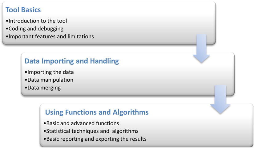
Figure 3-1. Three phases in learning SAS fundamentals
This chapter will focus on manipulating data in SAS. You’ll learn about SAS data sets, SAS libraries, and SAS statement, import data, and you’ll learn how to import data, use SAS constructs such as if-then-else, create new variables, and so on. All of these are fundamental tools for working with SAS.
A SAS data set contains two main portions. First is the descriptive portion of the data, which is similar to the metadata for a typical data set. Another is the data potion, which contains the usual rows and columns containing data typical in a two-dimensional table. In this book, whenever we write data set, we refer to the data portion. SAS data sets have a .sas7bdat extension, and you can open them in the SAS environment.
You are already probably familiar with many other formats for storing data. Examples of common storage are text files (.txt) and comma-separated files (.csv). In addition to working with SAS data, you will also learn how to read data from external files, later in this chapter.
Descriptive Portion of SAS Data Sets
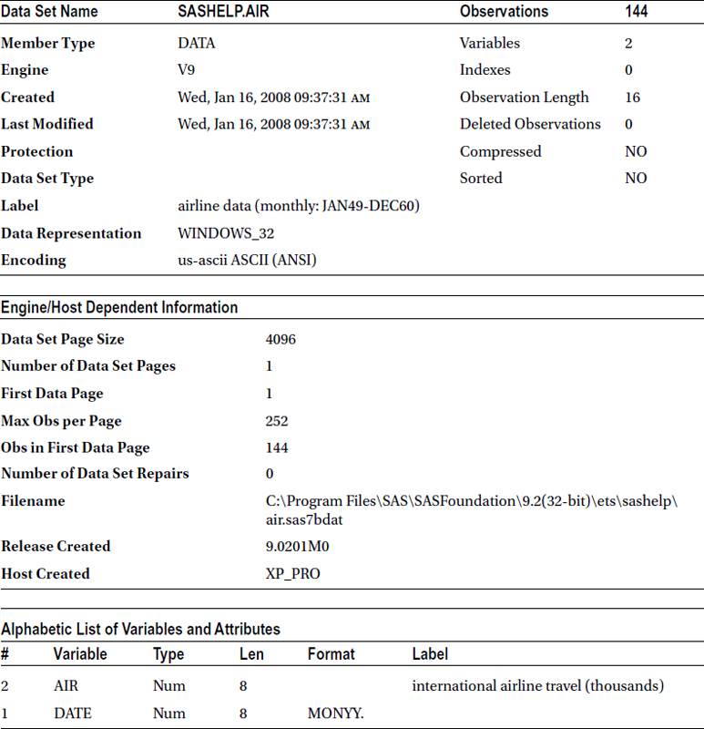
The descriptive portion of a data set contains the metadata, which is data about the data. This is mainly the description of variables and of the data set contained in the SAS data set. You can use the simple contents procedure in SAS (PROC CONTENTS) to get this metadata. The descriptive portion contains details such as when the data set was created, where it is stored, how many variables and observations it contains, the data type of variables, and so on. Given next is an example that shows the code and output (Table 3-1) associated with PROC CONTENTS. It prints the descriptive portion of the air data set from the sashelp library.
proc contents data=sashelp.air;
run;
Table 3-1. The CONTENTS Procedure
Dealing with the data potion of data sets is fortunately pretty simple in SAS. As discussed earlier, the data portion in SAS data sets contains the data rows (more appropriately called observations or records) and datelines along with the columns (called variables). You can use the print procedure of SAS (PROC PRINT) to see the data set. The following is the SAS code for printing the first ten observations of the sashelp.air data set:
proc print data=sashelp.air(obs=10);
run;
Table 3-2 lists the output of this code.
Table 3-2. Output of PROC PRINT on the sashelp.air Data Set
|
Obs |
DATE |
AIR |
|---|---|---|
|
1 |
JAN49 |
112 |
|
2 |
FEB49 |
118 |
|
3 |
MAR49 |
132 |
|
4 |
APR49 |
129 |
|
5 |
MAY49 |
121 |
|
6 |
JUN49 |
135 |
|
7 |
JUL49 |
148 |
|
8 |
AUG49 |
148 |
|
9 |
SEP49 |
136 |
|
10 |
OCT49 |
119 |
As a quick recap, Table 3-3 lists the frequently used file icons and extensions in SAS environments.
Table 3-3. Commonly Used File Icons and Extensions in the SAS Environment


SAS data sets are stored in SAS libraries. The previous example used the air data set from the sashelp library. Every data set is best stored in a library first; otherwise, you wouldn’t be able to work with it in the SAS environment. Just to summarize,
- A SAS library is a collection of SAS data sets and other SAS files.
- You can, for example, create a SAS library from an Oracle database containing tables.
You need to define a library to be able to store any data set. A SAS library is not a virtual folder; it is a physical folder in the Windows environment. You just refer to the physical path of a library and the physical folder’s name using a handle (the library name). So, while creating a library, you need to give two mandatory parameters, the library name and the physical path, where the files will be stored. Described next are the two ways to create a new library: using a graphical user interface (GUI) and using SAS code.
Creating the Library Using the GUI
SAS provides a GUI to create and work with libraries. Here are the steps for creating a library:
- Open Explorer (Figure 3-2).

Figure 3-2. Creating a new library: opening Explorer
- Double click the Libraries folder icon. This folder contains all the default libraries in SAS (Figure 3-3).

Figure 3-3. Creating a new library: The active libraries
- Right-click within the Explorer window and select New to create a new library (Figure 3-4).
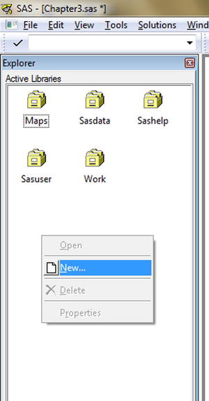
Figure 3-4. Creating a new library: right-click and select the New menu option
- Give the library a name (Figure 3-5).
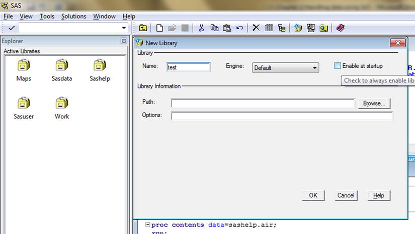
Figure 3-5. Creating a new library: filling in the library name
- Give the physical path of the library (Figure 3-6). All the data sets stored in the library can be seen in that location.

Figure 3-6. Creating a new library: fill in the physical path of the library
- Click OK, and the new library will be created (Figure 3-7).
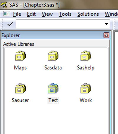
Figure 3-7. Creating a new library: the new library Test is created
Obviously, the newly created library is empty as of now. You can verify this by double-clicking the Test icon (Figure 3-8).
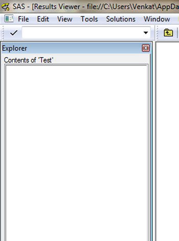
Figure 3-8. Creating a new library: the new library Test
What happens if you follow the same steps and create a new library named 1temp (Figure 3-9)?
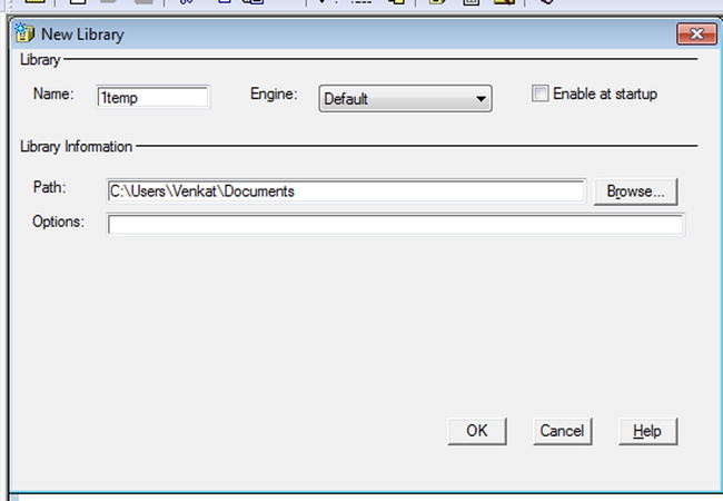
Figure 3-9. Creating a new library: an invalid name
The library will not be created because 1temp is an invalid name; you will get the error given in Figure 3-10.
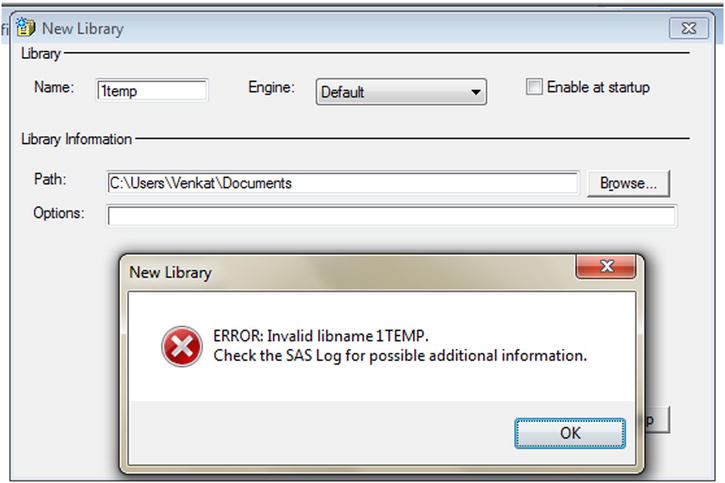
Figure 3-10. Creating a new library: error, showing an invalid name
You cannot use a random string as a library name. There are certain naming rules while creating the library, covered next.
The rules for defining the library name are as follows:
- The maximum length of the library name is eight characters long.
- The library name must start with a letter or underscore only.
- The library name can be a combination of letters, numbers, and underscores.
Table 3-4 lists some example library names that work and also some library names that throw an error.
Table 3-4. Valid and Invalid SAS Library Names
|
Library Name |
Result |
Comment |
|---|---|---|
|
Mylib |
Works |
The library name is less than eight characters long. |
|
Mylib1 |
Works |
The library name is a combination of letters and numbers. |
|
$Mylib |
Throws an error |
The library name cannot start with a special character other than an underscore (_). |
|
_Mylib |
Works |
The library name can start with an underscore (_). |
|
Mylib$ |
Throws an error |
The library name cannot have any special character other than an underscore (_). |
|
_mylib_ |
Works |
A library name can include an underscore (_). |
|
2mylib |
Throws an error |
The library name cannot start with a number. |
|
Datalib2013Sales |
Throws an error |
The library name is too long. It cannot have more than eight characters. |
Creating a New Library Using SAS Code
The SAS code for creating a new library follows:
libname <Library name> '<Library path>';
 libname mydata 'C:UserssalesDesktopData';
This code will create a library called mydata, and it will be attached to the following folder:
C:UserssalesDesktopData
Here is the log message when you execute the preceding code:
22   libname mydata 'C:UserssalesDesktopData';
NOTE: Libref MYDATA was successfully assigned as follows:
      Engine:        V9
      Physical Name: C:UserssalesDesktopData
Permanent and Temporary Libraries
There are two types of libraries in SAS: permanent and temporary. The libraries you created by using the libname statement and the GUI are permanent libraries. Once a data set is created in a permanent library, you can use it in the future, and the data set will be available even after a system reboot. By creating or importing a data set into a permanent library, you are physically creating a permanent data set.
Work is a temporary library in SAS. The data sets created in the Work library last only for the current SAS session. Once you close and reopen SAS, all the data sets in the Work library will be lost. If you don’t specify any library name with a data set, then, by default, SAS stores the data set in Work.
Let’s explore these concepts in more depth with an exercise. The following code creates a data set with two columns. You will use this code to create a data set in Work as well as in a permanent library called Mydata. You then close and reopen SAS to see whether the data set is still there.
The following code creates an Income data set in the mydata library with two variables: income and expense. You also put some records the income data set using the datalines keyword.
data mydata.income;
input income expense;
datalines;
4500 2000
5000 2300
7890 2810
8900 5400
2300 2000
;
run;
The log messages when this code is executed look like this:
NOTE: The data set MYDATA.INCOME has 5 observations and 2 variables.
NOTE: DATA statement used (Total process time):
      real time           0.07 seconds
      cpu time            0.01 seconds
Figure 3-11 shows the contents of the library Mydata. You can see an Income icon, which is the recently created data set.
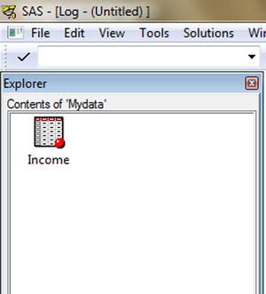
Figure 3-11. Contents of the Mydata library
The following code creates the Income data set in the Work library with the same details as you did for the Mydata library:
data work.income;
input income expense;
datalines;
4500 2000
5000 2300
7890 2810
8900 5400
2300 2000
;
run;
The log messages when you execute this code look like this:
NOTE: The data set WORK.INCOME has 5 observations and 2 variables.
NOTE: DATA statement used (Total process time):
      real time           0.01 seconds
      cpu time            0.01 seconds
Figure 3-12 shows the contents of the library Work. You can see the Income icon, which is the recently created data set.
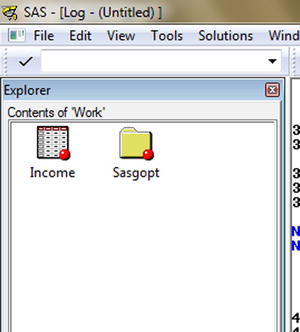
Figure 3-12. Contents of Work library after creating the Income data set
The following code also creates Income data set in the Work library. If you don’t mention any library name, the data set will be created in Work, by default.
Data income;
input income expense;
datalines;
4500 2000
5000 2300
7890 2810
8900 5400
2300 2000
;
run;
If you close SAS and reopen it, then you will not be able to see the Income data set in the Work library. By contrast, in Mydata, you will observe that the Income data set is still available.
![]() Note If the Mydata library vanishes or gets deleted from the library list, it may not be a reason for worry. All you need to do is rerun the following code to re-create just the library name and assign it the directory path. After doing so, you will again see the Income data set in Mydata. You need not create the data set again. The data set, Income, is permanently created in the given library folder path with a file extension of .sas7bdat.
Note If the Mydata library vanishes or gets deleted from the library list, it may not be a reason for worry. All you need to do is rerun the following code to re-create just the library name and assign it the directory path. After doing so, you will again see the Income data set in Mydata. You need not create the data set again. The data set, Income, is permanently created in the given library folder path with a file extension of .sas7bdat.
libname mydata 'C:UserssalesDesktopData';
Now that you’ve learned how to work with SAS libraries, it’s time to learn about the basics of SAS coding, which will allow you to work with data and perform some meaningful analysis. The following section introduces you to SAS PROC and DATA steps, the most basic building blocks of writing SAS code.
Two Main Types of SAS Statements
There are two main types of SAS statements (see Table 3-5). One starts with DATA, and the other one starts with PROC. The data step is mainly used for variable creation, data manipulation, and other data-related operations. The PROC step is used for calling (in the SAS code) various algorithms, special functions, and so on. PROC stands for the word procedure, which means prewritten code in SAS.
Table 3-5. DATA Step and PROC Step
|
DATA Step |
Proc Step |
|---|---|
|
Starts with a keyword DATA. Used for data manipulations. Creating calculated fields. Mainly used in reporting. Data merging, joining, data cleaning operations. Example: Preparing the data for analysis, from the orginal raw data, requires lot of data operations. |
Starts with keyword PROC. Used for analysis and other complex operations. You can create the data sets by taking the output of PROC step. Example: Predicting the sales by using regression algorithm needs PROC REG. |
Before you can start working on data, you need to import it into a SAS library in the form of SAS data sets. The data can be imported into SAS from many sources such as CSV files, Excel files, TXT files, database files, and so on. The following sections explain some ways of importing into and creating the data in SAS.
Data Set Creation Using the SAS Program
If you have to create a small data set based on some data provided to you, you create it by writing a small SAS program.
Here is a sample program to create a data set:
data mydata.income;
input income expense;
datalines;
4500 2000
5000 2300
7890 2810
8900 5400
2300 2000
;
run;
Given in Table 3-6 is the explanation of the preceding syntax.
Table 3-6. Program Syntax Explanation
|
SAS Statement |
Explanation |
|---|---|
|
data |
This is a keyword to create a new data set in SAS. |
|
mydata.income; |
Mydata is the library name, and income is the new data set name. |
|
input |
This is a keyword for declaring the variables in the data. |
|
income expense; |
These are two variables that will be created in the new data set. |
|
datalines; |
This is a keyword for entering the data into the data set. |
|
4500 2000 5000 2300 7890 2810 8900 5400 2300 2000 ; |
This is the actual data. |
Here is the log file when you execute this program:
NOTE: The data set MYDATA.INCOME has 5 observations and 2 variables.
NOTE: DATA statement used (Total process time):
      real time           0.03 seconds
      cpu time            0.03 seconds
Figure 3-13 shows the Income data set in the Mydata library.
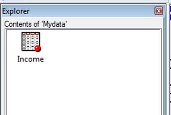
Figure 3-13. Contents of the Mydata library after creating the Income data set
Generally, the data set creation step is useful when you quickly want to create a small data set to use in the analysis. If you are creating really large data sets, then manually entering the values is obviously not the desired option. You need to use SAS import features for bringing large data files into the SAS environment.
Using the Import Wizard
You can import the data from external files into SAS by writing SAS code, or you can use the Import Wizard. Let’s first look at how to import the external flat files into SAS using the Import Wizard. Here are the steps to import the data:
- Select: File
 Import Data (see Figure 3-14).
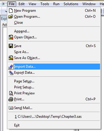
Figure 3-14. Importing data: select the Import Data option
- Select the type of file. In this example, you are going to import a CSV file; hence, you select the CSV format (see Figure 3-15 and Figure 3-16).
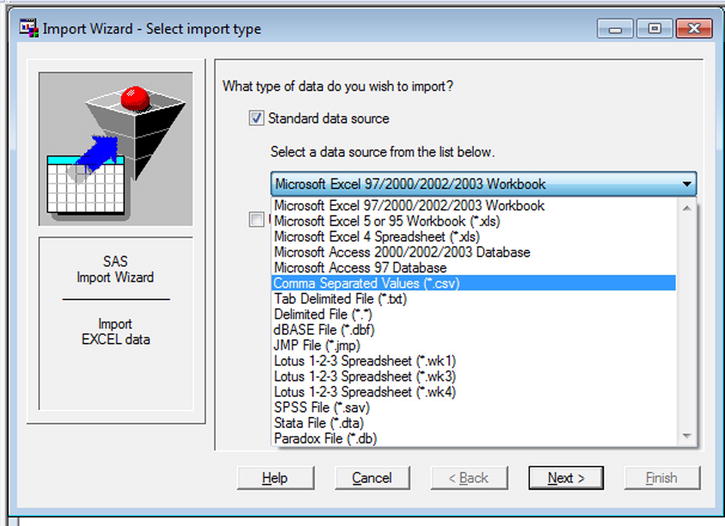
Figure 3-15. Importing data: select the file type
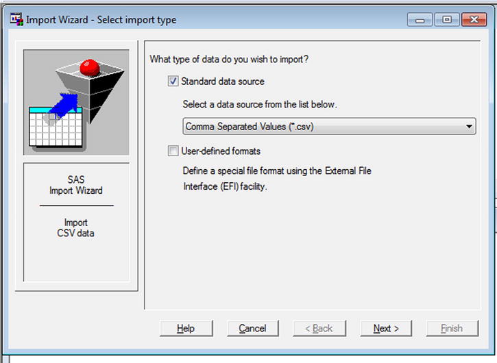
Figure 3-16. Importing data: the final selection screen
- Click Next.
- Locate the input file using the Browse button (see Figure 3-17).
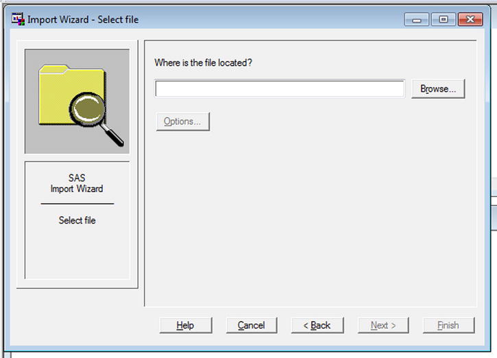
Figure 3-17. Importing data: browse to the file location
Figure 3-18 shows the wizard with the proper file path entered.
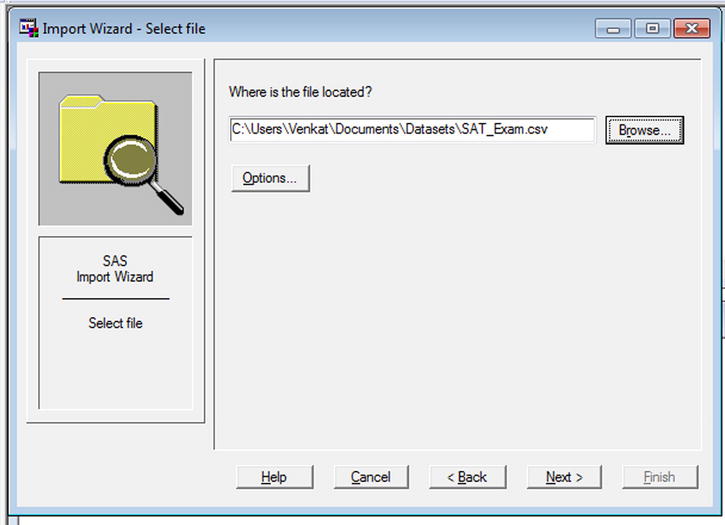
Figure 3-18. Importing data: the file folder path being selected
- Select the file and click Next.
- Give the details of the destination SAS data set (see Figure 3-19).
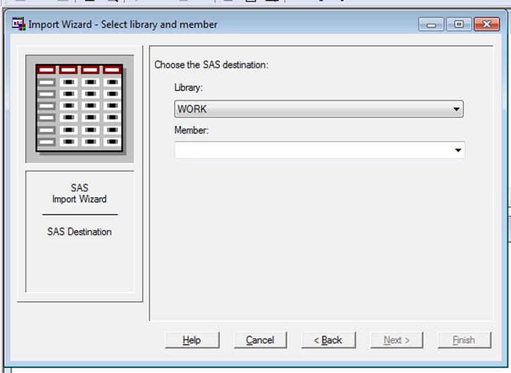
Figure 3-19. Importing data: SAS data set destination details
- Choose the library (see Figure 3-20).
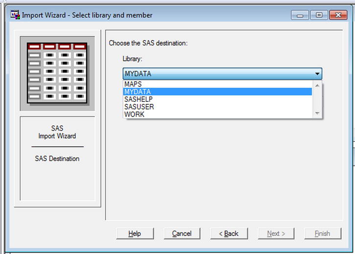
Figure 3-20. Importing data: choose the library
- Name the target data set (see Figure 3-21).
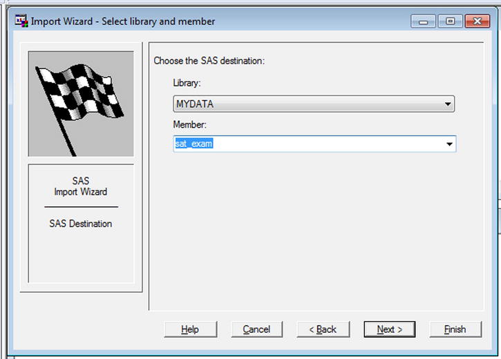
Figure 3-21. Importing data: name the target data set
- If you think you will want to import this data again, you can save the importing steps to a SAS file (see Figure 3-22). This step is optional. Browse to a location and save the .sas file (see Figure 3-23).
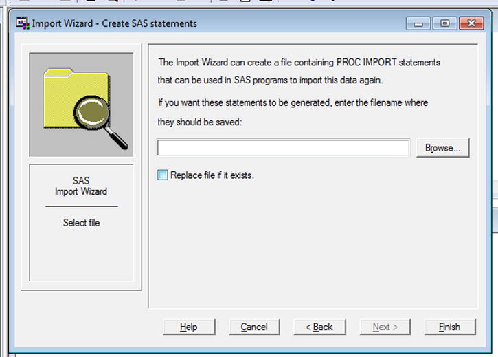
Figure 3-22. Importing data: the option to generate and save the code for import GUI options
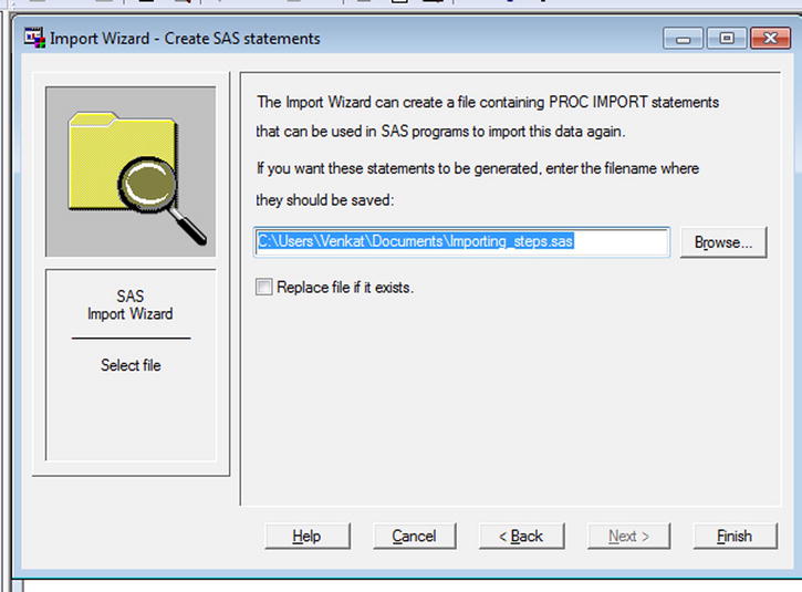
Figure 3-23. Importing data: generate and save the code for import GUI options in a .sas file
- Click Finish to end the process.
The data set will be in the library, and the SAS code will be in the .sas file. Figure 3-24 shows the sat_exam data set stored in the Mydata library.
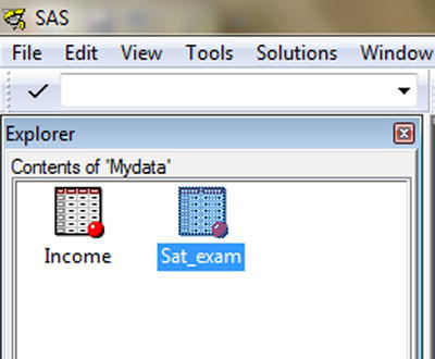
Figure 3-24. Importing data: contents of the Mydata library
The SAS code from the file you saved follows:
PROC IMPORT OUT= MYDATA.sat_exam
            DATAFILE= "C:UsersDocumentsDatasetsSAT_Exam.csv"
            DBMS=CSV REPLACE;
     GETNAMES=YES;
     DATAROW=2;
RUN;
In the same fashion, you can import different types of files such as TXT files, Excel files, and so on, using the Import Wizard. The next section explains the SAS code to import the data.
Import Using the Code
In the previous section you imported data using the GUI. You can also import data using SAS code. While analyzing data, usually some data manipulation code is also need after the data import, so it’s convenient that you write the data import code in the same file.
Importing a CSV File Using Code
The following code imports a simple CSV file into SAS:
PROC IMPORT OUT= MYDATA.sat_exam
            DATAFILE= "C:UsersDocumentsDatasetsSAT_Exam.csv"
            DBMS=CSV REPLACE;
     GETNAMES=YES;
     DATAROW=2;
RUN;
Table 3-7 explains this code.
Table 3-7. Code to Import a .csv File
|
SAS Statement |
Explanation |
|---|---|
|
PROC IMPORT |
This is the procedure for importing data into SAS. |
|
OUT= MYDATA.sat_exam |
This is the OUT keyword for mentioning the output file in SAS. Here you are importing and storing the data set as sat_exam in the Mydata library. |
|
DATAFILE= "C:UsersDocumentsDatasetsSAT_Exam.csv" |
The DATAFILE keyword is for mentioning the input data file that needs to be imported into SAS. You need to specify the full folder path of the file along with extension. |
|
DBMS=CSV |
DBMS=CSV indicates the type of file you are importing. |
|
REPLACE; |
If there is already a file with the same name as MYDATA.sat_exam, then this option will replace that file. Note that the first SAS statement ends here, and there is no semicolon until here. |
|
GETNAMES=YES; |
Get the column names from import file? Yes or No? |
|
DATAROW=2; |
Where is the data starting from? In this case, the first row is the column names, and the data is starting from the second row. |
Here is the code for importing a CSV file containing burger sales:
 PROC IMPORT OUT= MYDATA.burger
            DATAFILE= "C:UsersDocumentsDatasetsBurger_sales.csv"
            DBMS=CSV REPLACE;
     GETNAMES=YES;
     DATAROW=2;
RUN;
The important notes from the log file when you execute this code follows:
NOTE: The infile 'C:UsersDocumentsDatasetsBurger_sales.csv' is:
      Filename=C:UsersDocumentsDatasetsBurger_sales.csv,
      RECFM=V,LRECL=32767,File Size (bytes)=375,
      Last Modified=10Jun2014:15:33:18,
      Create Time=05Oct2014:17:02:57

NOTE: 35 records were read from the infile 'C:UsersDocumentsDatasetsBurger_sales.csv'.
      The minimum record length was 8.
      The maximum record length was 9.
NOTE: The data set MYDATA.BURGER has 35 observations and 2 variables.
NOTE: DATA statement used (Total process time):
      real time           0.03 seconds
      cpu time            0.03 seconds

35 rows created in MYDATA.BURGER                             from
C:UsersDocumentsDatasetsBurger_sales.csv.

NOTE: MYDATA.BURGER data set was successfully created.
NOTE: PROCEDURE IMPORT used (Total process time):
      real time           0.10 seconds
      cpu time            0.10 seconds
Let’s look at how to import other types of files.
Importing an Excel File Using SAS Code
There is an additional parameter RANGE in the following Excel import code. This refers to a worksheet name in an Excel sheet. Generally an Excel file has multiple worksheets, so you need to mention the sheet that needs to be imported.
PROC IMPORT OUT= MYDATA.BURGER_sales_from_excel
            DATAFILE= "C:UsersDocumentsDatasetsBurger_sales.xls"
            DBMS=EXCEL REPLACE;
     RANGE="Burger_sales$";
     GETNAMES=YES;
   RUN;
Here are the log messages when you execute this code:
153  PROC IMPORT OUT= MYDATA.BURGER_sales_from_excel
154              DATAFILE= "C:UsersDocumentsDatasetsBurger_sales.xls"
155              DBMS=EXCEL REPLACE;
156       RANGE="Burger_sales$";
157       GETNAMES=YES;
158     RUN;

NOTE: MYDATA.BURGER_SALES_FROM_EXCEL data set was successfully created.
NOTE: PROCEDURE IMPORT used (Total process time):
      real time           0.13 seconds
      cpu time            0.06 seconds
Similarly, the following code imports a text file:
PROC IMPORT OUT= MYDATA.SAT_EXAM_data_from_text_file
            DATAFILE= "C:UsersDocumentsDatasetsSAT_Exam.txt"
            DBMS=TAB REPLACE;
     GETNAMES=YES;
     DATAROW=2;
RUN;
You can import various types of files using PROC IMPORT; the only change is in some of the parameters in the import code.
You import raw data using the import code. Most of the time you need to manipulate the raw data to prepare it for analysis. In the process, you may have to subset the data, merge it with a different data set, create new calculated variables, derive variables from existing variables, and so on. The following sections take you through some important steps, which you will need while manipulating data for almost any analysis.
Making a Copy of a SAS Data Set
Imagine that you have imported some data and you further want to prepare the data for analysis. The following code creates a copy of the data set in SAS. For this, you use a SET statement in the data step:
data MYDATA.sat_exam_copy;
set  MYDATA.sat_exam;
run;
The preceding code simply copies the data from sat_exam and stores it in sat_exam_copy in the MYDATA library. Here is the log file for this code:
NOTE: MYDATA.SAT_EXAM_DATA_FROM_TEXT_FILE data set was successfully created.
NOTE: PROCEDURE IMPORT used (Total process time):
      real time           0.60 seconds
      cpu time            0.18 seconds

1761  data MYDATA.sat_exam_copy;
1762  set  MYDATA.sat_exam;
1763  run;
NOTE: There were 96 observations read from the data set MYDATA.SAT_EXAM.
NOTE: The data set MYDATA.SAT_EXAM_COPY has 96 observations and 5 variables.
NOTE: DATA statement used (Total process time):
      real time           0.03 seconds
      cpu time            0.01 seconds
Similarly, if you want to copy the data set into a different library, say Work, then you can use the following code:
data sat_exam_copy;
set  MYDATA.sat_exam;
run;
Here is the log file for this code:
NOTE: There were 96 observations read from the data set MYDATA.SAT_EXAM.
NOTE: The data set MYDATA.SAT_EXAM_COPY has 96 observations and 5 variables.
NOTE: DATA statement used (Total process time):
      real time           0.03 seconds
      cpu time            0.03 seconds
Let’s use an example of a market campaign’s data to understand this topic better. The following code imports the market data file:
PROC IMPORT OUT= MYDATA.market
            DATAFILE= "C:UsersDocumentsDatasetsMarket_campaign.csv"
            DBMS=CSV REPLACE;
     GETNAMES=YES;
     DATAROW=2;
RUN;
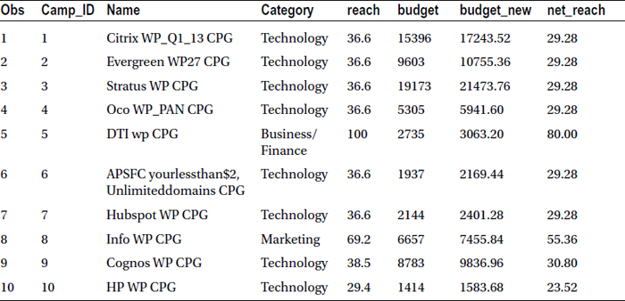
Table 3-8 lists the snapshot of the market campaign data.
Table 3-8. A Snapshot of the Market Campaign Data
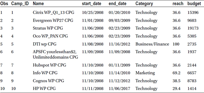
Table 3-9 lists the variables and their descriptions.
Table 3-9. The Variables and Their Descriptions for Market Data Examples
|
Variable |
Description |
|---|---|
|
Camp_id |
Market campaign ID |
|
name |
Name of the market campaign |
|
start_date |
Campaign start date |
|
end_date |
Campaign end date |
|
Category |
Category or type of campaign |
|
reach |
Campaign reach (100 percent reach is the target) |
|
budget |
Market campaign budget |
In the next section, you will use this market campaign case study to try various data manipulation operations using SAS.
To create a new variable, you, once again, use a set statement along with new variable statement. Here is a generic sample:
data new_data;
set old_data;
<new var statements>;
run;
Let’s try to write some actual SAS code snippets to elaborate on the previous generic code to create new variables.
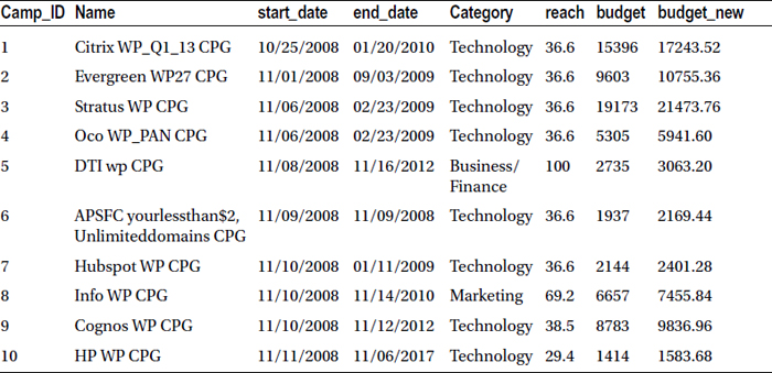
Create a new variable, budget_new, by adding 12 percent tax.
data MYDATA.market_v1;
set MYDATA.market;
budget_new=budget*1.12;
run;
The log file for the preceding code follows:
NOTE: There were 7843 observations read from the data set MYDATA.MARKET.
NOTE: The data set MYDATA.MARKET_V1 has 7843 observations and 8 variables.
NOTE: DATA statement used (Total process time):
      real time           0.01 seconds
      cpu time            0.01 seconds
Note the first line of the SAS log file. It translates as follows. Whenever a record has a missing value of budget, the budget_new variable will also have a missing value. This is an important point to be remembered while dealing with data in SAS.
Table 3-10 lists the snapshot of the new data set, market_v1.
Table 3-10. A Snapshot of the New Data Set: market_v1
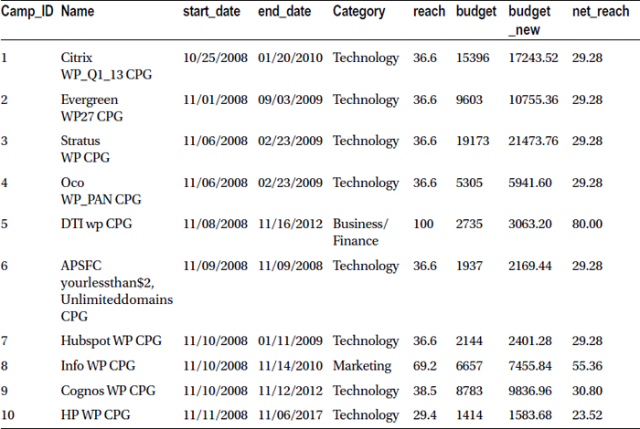
Let’s suppose that the reach values are inflated. Take only 80 percent of the reach and name the new variable net_reach, as shown here:
data MYDATA.market_v2;
set MYDATA.market_v1;
net_reach=reach*0.8;
run;
Here is the log file for this code:
NOTE: There were 7843 observations read from the data set MYDATA.MARKET_V1.
NOTE: The data set MYDATA.MARKET_V2 has 7843 observations and 9 variables.
NOTE: DATA statement used (Total process time):
      real time           0.01 seconds
      cpu time            0.01 seconds
Table 3-11 lists the snapshot of the new data set, market_v2.
Table 3-11. A Snapshot of the New Data Set, market_v2
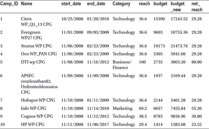
In fact, you can execute both operations in the same data step as follows:
Data MYDATA.market_v3;
set MYDATA.market;
budget_new=budget*1.12;
net_reach=reach*0.8;
run;
Here is the log file for this code:
NOTE: There were 7843 observations read from the data set MYDATA.MARKET.
NOTE: The data set MYDATA.MARKET_V3 has 7843 observations and 9 variables.
NOTE: DATA statement used (Total process time):
      real time           0.01 seconds
      cpu time            0.01 seconds
Table 3-12 lists the snapshot of the new data set, market_v3.
Table 3-12. A Snapshot of the New Data Set, market_v3
Creating New Variables Using Multiple Variables
The syntax for creating a new field in a table using multiple variables is similar to what you have already seen for creating a single variable. The following is the generic code:
data new_data;
set old_data;
<new var statements>;
run;
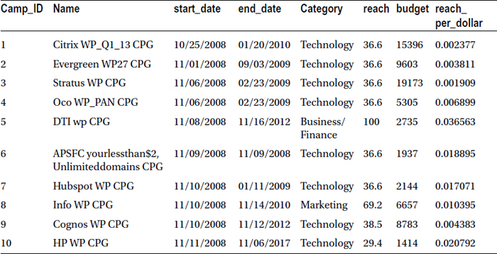
Let’s look at an example: A market campaign’s effectiveness is measured by its reach with respect to the budget. Reach per dollar is the new variable that you want to create to determine the effectiveness of each campaign. Here is the code:
Data MYDATA.market_v4;
set  MYDATA.market;
reach_per_dollar=reach/budget;
run;
Table 3-13 lists the snapshot of the new data set, market_v4.
Table 3-13. A Snapshot of the New Data Set, market_v4
Creating New Variables Using if-then-else
You might have to use an if-then-else structure to create new categorical variables that contain values such as High, Medium, Low, Yes or No, and so on. The following is the generic syntax for creating variables using an if-then-else structure:
data new_data;
set old_data;
<if then else statements>;
run;
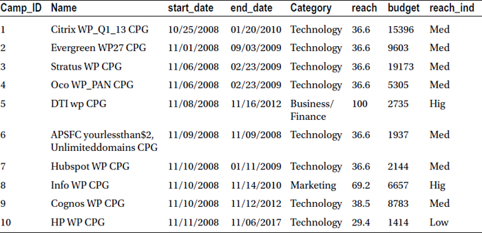
Again, let’s look at an example: Create a new variable called reach_ind (reach indicator), which takes a value of High when the reach is more than 66 percent, Medium when the reach is in between 33 percent and 66 percent, and Low when the reach is less than 33 percent.
Data MYDATA.market_v5;
set  MYDATA.market;
if reach<33 then reach_ind='Low';
else if reach >= 33 and reach <=66 then reach_ind='Med';
else reach_ind='High';
run;
Table 3-14 lists the snapshot of the new data set, market_v5.
Table 3-14. A Snapshot of the New Data Set, market_v5
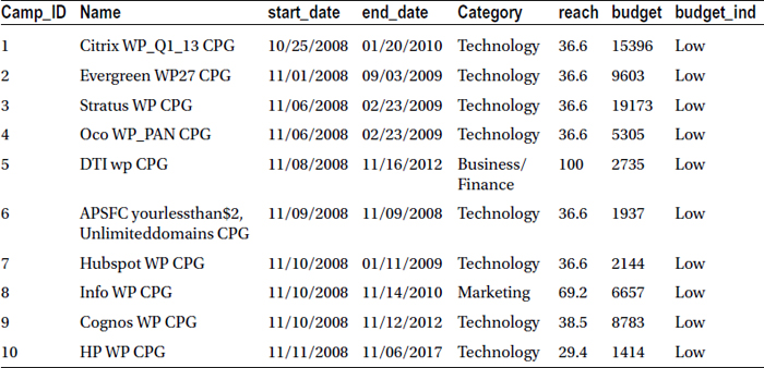
Here is another example. Create a new variable called budget indicator, which takes a value of High when the budget is more than 75000, Medium when the reach is in between 20000 and 75000, and Low when the reach is less than 20000.
Data MYDATA.market_v6;
set  MYDATA.market;
if budget<20000 then budget_ind='Low';
else if budget >= 20000 and budget <=75000 then budget_ind='Med';
else budget_ind='High';
run;
Table 3-15 lists the snapshot of the new data set, market_v6.
Table 3-15. A Snapshot of the New Data Set, market_v6
Until now, you have seen how to create a new data set by adding a new variable to the original one. If the situation demands, you can add new variables to the same data set. Here is the generic code:
data old_data;
set old_data;
<New variable statements>;
run;
The following example updates the market data while creating budget_new and net_reach variables:
Data MYDATA.market;
set MYDATA.market;
budget_new=budget*1.12;
net_reach=reach*0.8;
run;
Table 3-16 lists the snapshot of the updated data set (market).
Table 3-16. A Snapshot of the Updated Data Set (market)

Sometimes you might not need all the variables from a raw data set. On a few occasions, you might want to keep some important variables and delete the ones that are not relevant to the analysis. For example, you may want to keep just 10 important variables out of a list of 200 in the raw data set. The syntax of this “keep and drop” SAS construct follows:
Syntax for Keep
data new_data;
set old_data(Keep=Var1 Var2 Var3);
<Rest of the statements>
run;
Syntax for Drop
data new_data;
set old_data(Drop=Var5 Var6 Var7);
<rest of the statements>
run;
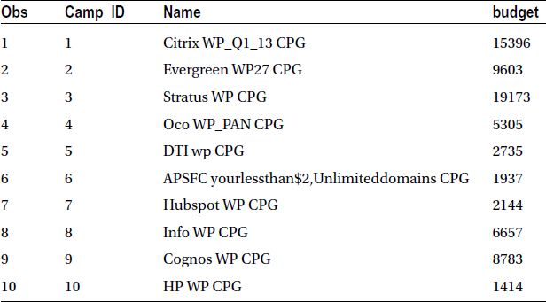
In this first example, you create a new data set from the market data; keep only the campaign ID, the name, and the budget. The idea is to perform a univariate analysis solely on budget. You will learn about univariate analysis in later chapters.
Data MYDATA.market_v7;
set MYDATA.market(keep=camp_id name  budget);
run;
Table 3-17 lists the snapshot of the updated data set (market_v7).
Table 3-17. A Snapshot of the Updated Data Set (market_v7)
In this second example, you create a new data set from the market data, with the drop start date and end date. They will not be used anywhere in the analysis.
Data MYDATA.market_v8;
set MYDATA.market(Drop=start_date end_date);
run;
Table 3-18 lists the snapshot of the updated data set (market_v8).
Table 3-18. A Snapshot of the Updated Data Set (market_v8)
These are examples of dropping the fields or columns or variables from the data. Now you will see how to subset or filter the data, that is, using some specific rows based on a condition.
Subsetting or filtering is almost an inevitable operation while manipulating the data. You may not need all the rows of raw data for analysis. You may just want to filter out irrelevant data and consider only the data relevant for the further analysis. You are going to use the same set statement again. Here is the generic code:
data new_data;
set old_data;
<Where condition>;
run;
Here is another example:
data new_data;
set old_data;
<if condition>;
run;
In this example, you extract a subset from the market data. The resultant data should contain campaigns from the healthcare category only. The following code fulfills this requirement:
Data MYDATA.market_v9;
set MYDATA.market;
where category='Healthcare';
run;
or
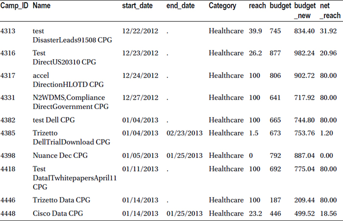
Data MYDATA.market_v10;
set MYDATA.market;
if category='Healthcare';
run;
Table 3-19 lists the snapshot of the updated data set (market_v9).
Table 3-19. A Snapshot of the Updated Data Set (market_v9)
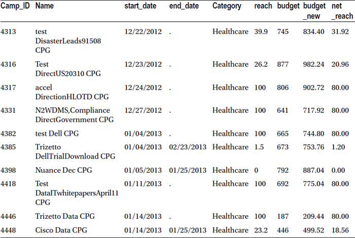
Table 3-20 lists the snapshot of the updated data set (market_v10).
Table 3-20. A Snapshot of the Updated Data Set (market_v10)
To subset the data, you can use either a where or an if condition. Yes, there is a difference between using the two conditions, even though the resulting data set appears to be the same.
Differences Between where and if
To understand the difference, you need to take a closer look at the log messages (Table 3-21).
Table 3-21. Differences Between where and if Clauses
|
Where Condition |
If Condition |
|---|---|
|
NOTE: There were 112 observations read from the data set MYDATA.MARKET. WHERE category ='Healthcare'; NOTE: The data set MYDATA.MARKET_V9 has 112 observations and 7 variables. NOTE: DATA statement used (Total process time): real time 0.03 seconds cpu time 0.01 seconds |
NOTE: There were 7843 observations read from the data set MYDATA.MARKET. NOTE: The data set MYDATA.MARKET_V10 has 112 observations and 7 variables. NOTE: DATA statement used (Total process time): real time 0.01 seconds cpu time 0.00 seconds |
|
The where clause reads only 112 observations. |
The if clause reads complete data set into SAS. |
|
The where clause first applies the filter and then reads the observations. |
The if clause reads all the records and then applies the filters. |
|
Even when there are 100,000,000 observations (for example), the where condition will apply the filter first and then read the remaining records, so it is fast compared to an if condition. |
When there are 100,000,000 observations (for example), it will take lot of time to read all of them into SAS and then start applying the filters, so it takes more time compared to the where condition. |
|
The where clause works not only in the data step; it works in the PROCstep also. proc print data= MYDATA.market; where category='Healthcare'; run; The previous code successfully prints healthcare data. |
If works only in the data step; it doesn’t works in the PROC step. proc print data= MYDATA.market; if category='Healthcare'; run; This code generates the error, given below 580 proc print data= MYDATA.market; 581 if category='Healthcare'; -- 180 ERROR 180-322: Statement is not valid or it is used out of proper order. 582 run; |
Conclusion
In this chapter, you learned the basic concepts related to data manipulation in the SAS programming environment. The chapter focused on how to handle data in SAS, how to import data into SAS, how to create derived variables, and how to create a subset of the data. These coding concepts are useful when preparing data for analysis.
In the next chapter, you will see some of the important SAS procedures and start working with them. You will also learn how to join various data sets.