
![]()
Important SAS Functions and Procs
In the previous chapter, you learned about some important data manipulation techniques. You will typically take the raw data and prepare it for analysis. Once the final data is ready, you can go ahead with the analysis. The analysis might involve representing simple aggregated tables in meaningful graphs, applying simple descriptive statistics to advanced analytics, and predictive modeling. You may need advanced algorithms and functions to perform the analysis. While learning an analytics tool, it’s vital to know how to use some of the important functions and algorithms.
In this chapter, you will learn about basic functions and important SAS procedures. The chapter discusses numeric, character, and date functions, as well as some important SAS procedures such as CONTENTS and SORT. Finally, you’ll learn about some graphic functions such as GCHART and GPLOT.
SAS has prewritten routines for most of the numerical, string, and date operations. They are called functions. Using functions in SAS is not very different from the other programing languages. In fact, it’s easier. You need to write the function name and pass some mandatory and optional parameters. As usual, you expect each function to come with parentheses. If there are no parameters expected for a certain function, then the function will have nothing in the parentheses, as in today().
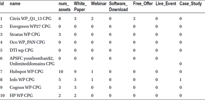
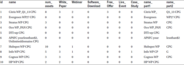
Let’s start with an activity to make some data ready for use later. Let’s import the Market_data_two data set, which will be used in several examples. This data set contains various types of assets used in typical marketing campaigns. Variables named White_Paper, Webinar, Software_Download, Free_Offer, Live_Event, and Case_Study represent different types of assets used for marketing campaigns.
The following SAS code imports and prints a snapshot of the data:
PROC IMPORT OUT= WORK.market_asset
            DATAFILE= "C:Users DocumentsTrainingBooksContent4. SAS Programs and AnalyticsDatasetsMarket_data_two.csv"
            DBMS=CSV REPLACE;
     GETNAMES=YES;
     DATAROW=2;
RUN;

proc print data=market_asset(obs=10) noobs;
run;
Table 4-1 lists the result of this code.
Table 4-1. A Snapshot of the Market Asset Data
Now that the data set is ready, you will learn how to use functions.
Numeric functions perform arithmetic operations on numerical variables. The following sections provide some examples.
Numerical Function Example: Mean
In this example, the numerical SAS function returns the arithmetic mean of a given number of numeric variables or a given set of numbers. The mean that we’re talking about here is row-wise; it’s not the mean of a particular column. If the number of assets is the field name, then the mean (of the number of assets) in SAS returns the same result as the numeric value in the row, since it is a row-wise mean. The average or mean is usually calculated for more than one variable, and it appears in each row.
The syntax of a mean function is as follows:
MEAN (Var1, Var2, Var3...)
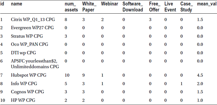
In this first example, you’ll determine, what is the average of two variables white paper and case study for each campaign. The following code finds the average. Here you will use the data set market_asset, created in the previous section.
Data market_asset_v1;
set market_asset;
mean_val=Mean(White_Paper, Case_Study);
run;

proc print data=market_asset_v1(obs=10) noobs;
run;
Table 4-2 lists the snapshot of the new data set with the mean value (mean_val) added as the last column.
Table 4-2. Mean of Variables White_Paper and Case_Study Added in the Last Column
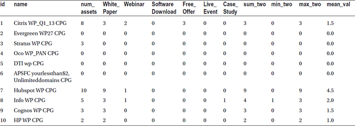
Here are a few more functions that are similar to the mean: sum, Min, and Max.
data market_asset_v2;
set market_asset;
sum_two=Sum(White_Paper,Case_Study);
min_two=min(White_Paper,Case_Study);
max_two=max(White_Paper,Case_Study);
mean_val=Mean(White_Paper, Case_Study);
run;

proc print data=market_asset_v2(obs=10)noobs;
run;
Table 4-3 contains a snapshot of the new data set, where the last four columns list the computed output from the SAS numeric functions.
Table 4-3. Numeric Functions Applied on the Variables White_Paper and Case_Study , Added in the Last Four Columns
In this second example, in the market asset data, the number of assets (num_assets) populated in the data set is supposed to be a simple sum of all assets: White_Paper, Webinar, Software_Download, Free_Offer, Live_Event, and Case_Study. An analyst claims that num_assets is not the exact sum. You need to verify this claim.
The following is the code along with the explanatory comments that the analyst writes to substantiate her claim:
/* introducing of a new dataset */

data market_asset_v3;

/* Using market_asset dataset */
set market_asset;

/* Finding sum of the columns in the dataset and storing it in num_asset_new*/

num_asset_new=Sum(White_Paper, Webinar, Software_Download, Free_Offer, Live_Event, Case_Study);

/* Finding the absolute difference between num_asset_new
and the column num_assets and storing it into Difference variable */

Difference=    abs( num_asset_new-num_assets);
run;

/* Printing first 10 observations of the dataset, where Difference is not equal to zero */

proc print data=market_asset_v3(obs=10) noobs;
where  Difference ne  0;
run;
For easier reading, the following is the same code without comments. Yes, SAS code files are really smaller than most other programming languages. The SAS code used throughout this book is similar, equal, or even lesser in size than this. Very cool!
data market_asset_v3;
set market_asset;
num_asset_new=Sum(White_Paper, Webinar, Software_Download, Free_Offer, Live_Event, Case_Study);
Difference=    abs( num_asset_new-num_assets);
run;

proc print data=market_asset_v3(obs=10) noobs;
where  Difference ne  0;
run;
Table 4-4 shows a snapshot of the new data set where the absolute difference is not equal to zero.
Table 4-4. Listing of the Data Set for the Second Example, Verifying the Analyst Claim
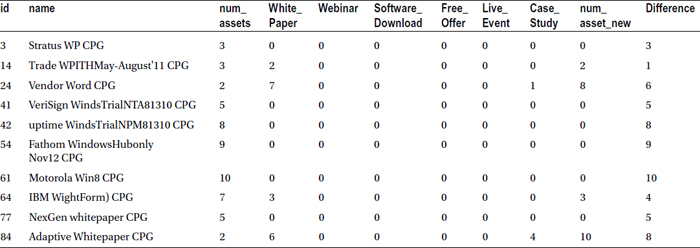
Table 4-5 lists some other commonly used numerical functions and their usage.
Table 4-5. Commonly Used SAS Numeric Functions
|
Function |
Feature |
Example |
|---|---|---|
|
LOG |
Returns the natural (base e) logarithm value |
x=log(5); y=log(2.2); z=log(x+y); |
|
EXP |
Returns the value of the exponential function |
x=exp(1); y=exp(0); z=exp(x*y); |
|
SQRT |
Returns the square root |
x=sqrt(14); y=sqrt(2*3*4); z=sqrt(abs (x-y)); |
|
N |
Returns the count of nonmissing values |
x=n(2,4,.); |
|
STD |
Returns the standard deviation of input variables |
y=std(2,4,.); |
|
VAR |
Returns the variance of the input variable |
z=var(2,4,.); |
|
INT |
Returns the integer value of the variable |
x1=int(543.210); |
Character or string functions are required to handle text variables. The following sections explain some of the commonly used character functions.
Substring
The substring function extracts a portion of a string variable. Imagine you want to use only the first four or five characters of a variable. The substring function will do the job for you.
Here is the syntax of the substring function:
New variable= SUBSTR(variable, start character, number of characters)
In this example, you take only the first ten characters of market campaign name (the name variable in the market_asset data set) and store them in the new variable name_part1. Once this is done, you take the next ten characters and store them in the variable name_part2.
Here is the code, which is self-explanatory:
data market_asset_v4;
set market_asset;
name_part1=substr(name,1,10); /* Substring first 10 characters */
name_part2=substr(name,11,10); /* Substring characters from 11 to 20 */
run;

proc print data=market_asset_v4(obs=10) noobs;
run;
;
Table 4-6 lists a snapshot of the new data set with two new string columns added at the end.
Table 4-6. A Snapshot of the Market Asset Data with Two New String Columns Added at the End
Here are some more string functions:
data  market_asset_v5;
set  market_asset;

/* LENGTH: returns an integer number, which is the position of the rightmost character in the string variable */

length_name=length(name);

/* TRIM: it removes trailing and following blanks. This function is useful for string concatenation */

trim_name=trim(name);

/* UPCASE: converts all lowercase letters in the string to uppercase letters */

Captial_name=Upcase(name);

/* LOWCASE: converts all uppercase letters in the string to lowercase letters */

Small_name=Lowcase(name);
run;

/* This print code lists the selected variables only */

proc print data=market_asset_v5(obs=10) noobs;
var id name length_name trim_name Captial_name    Small_name ;
run;

proc print data=market_asset_v5(obs=10) noobs;
var id name length_name trim_name Captial_name    Small_name ;
run;
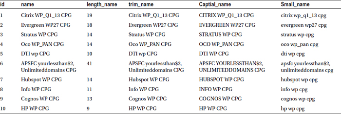
Table 4-7 lists the output of this code. You need to carefully observe the original string names in the second column and its transformations in the subsequent columns to comprehend what these functions are doing.
Table 4-7. Market Asset Data with Selected Variables, Application of String Functions
This section explains some commonly needed date functions that are used by the data analysts. Using date functions, you can manipulate date variables like formatting, finding durations in weeks and days, and so on.
You’ll often need to find the interval between two dates. It is not as simple as finding the difference (in number of days) between the start date and the end date. The difference may be required in days, months, years, and quarters. You can use the INTCK function to find the interval length between two dates.
This example again refers to the market campaign data set. It has a start date and an end date for each campaign. You need to find the duration of each campaign.
Here is the code:
data market_campaign_v1;
set market_campaign;
Duration_days=INTCK('day',start_date,end_date); /* Finds the duration in days */
Duration_months=INTCK('month',start_date,end_date); /* Finds the duration in months */
Duration_weeks=INTCK('week',start_date,end_date); /* Finds the duration in weeks */
run;

proc print data=market_campaign_v1(obs=10) noobs;
var camp_id name Duration_days  Duration_months Duration_weeks;
run;
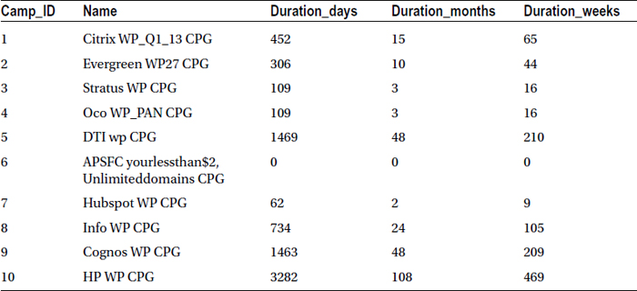
Table 4-8 gives the snapshot of the output.
Table 4-8. Campaign Duration Calculated in Days, Months, and Week Using the INTCK Function
The following are some more useful date functions:
data market_campaign_v2;
set market_campaign;

/* MONTH(date:returns the value as numeric for the month of the year for a SAS date */

start_month=month(start_date);

/* YEAR(date): returns the year from a valid SAS date */

start_year=year(start_date);
run;

proc print data=market_campaign_v2(obs=10) noobs;
run;
Table 4-9 is the snapshot of this code. The newly calculated start_month and start_year are added as the last two columns.
Table 4-9. Market Data Snapshot with Start Month and Year Calculated Using Date Functions

There are many more numeric, character, and date functions in SAS. Most of them are straightforward. They are not listed here, but you can easily Google them, as and when you need them.
In this section, you will see some of the important procedures (procs) in SAS. The data step is for data manipulations, and the proc, or procedure, step is for referring to algorithms and prewritten SAS routines. SAS procedures are useful for everything from producing simple data insights to getting inferences based upon advanced analysis.
The Proc Step
The proc step starts with the keyword PROC, and there is always a procedure name followed by the word PROC. You need to clearly understand the difference between functions and procedures in SAS. A function is a routine. In the following section, you start with a procedure by the name of PROC CONTENTS.
PROC CONTENTS
PROC CONTENTS gives you the SAS data set information that is similar to metadata of a database table. Before attempting to proceed with analysis, it is always a good idea to first look at the output of proc contents to get some quick information about data (or a data set to be precise). Contents data provides you with two levels of information.
- Data set level: This includes details of the data such as the name, total number of records, date created, number of variables, file size, file location and access permissions, and so on.
- Variable level: Details provided are the type of variable, length of variable, format of variable, and label of the variable.
Proc contents can be used for the following:
- Quickly checking the overall details of a data set instead of opening or printing it
- Checking the total number of observations after importing an external file into SAS
- Checking for a variable’s presence in a data set
- Verifying the type and format of a variable
PROC CONTENTS Example
The following code displays the contents of the Stocks data set from the sashelp library:
proc contents data=sashelp.stocks;
run;
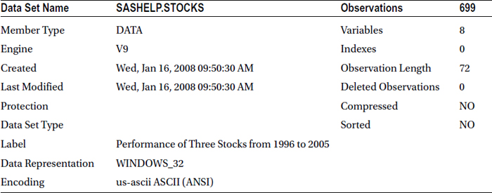
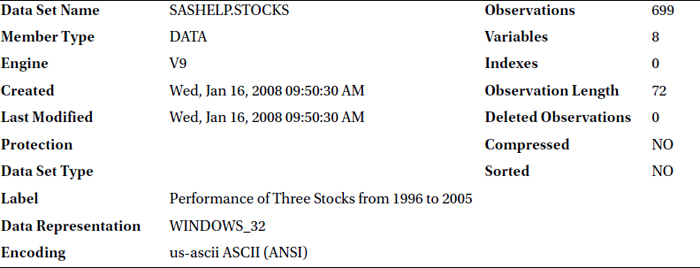
Table 4-10 lists the output of this SAS code.
Table 4-10. SAS Code Output of PROC CONTENTS on sashelp.stocks
|
Engine/Host Dependent Information | |
|---|---|
|
Data Set Page Size |
8192 |
|
Number of Data Set Pages |
7 |
|
First Data Page |
1 |
|
Max Obs per Page |
113 |
|
Obs in First Data Page |
86 |
|
Number of Data Set Repairs |
0 |
|
Filename |
C:Program FilesSASSASFoundation9.2(32-bit)graphsashelpstocks.sas7bdat |
|
Release Created |
9.0201M0 |
|
Host Created |
XP_PRO |
Here is the output of proc contents on the sashelp.stocks data set.
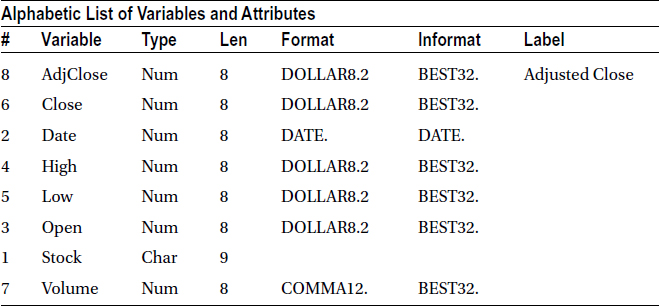
There are three tables in the output. The first one is all about the data set properties. The second table may be slightly less important from an analyst point of view. It lists how SAS stored this data. The third table, probably the most important one, is about variables in the data set and their properties.
Two useful options in PROC Contents are VARNUM and Short.
VARNUM Option
The variables in the Proc Contents output are printed in alphabetical order, not in the order in which they appear in the data set. To print them in the original order of data set, you use the varnum option. Here is the code using this option:
proc contents data=sashelp.stocks varnum;
run;
Table 4-11 lists the output of this code. You can see that the variables in the third table of this output are printed in the original order of the data set. This order is different from that of Table 4-10, which is alphabetical.
Table 4-11. The Output of proc contents on sashelp.stocks Data Set with varnum Option
|
Engine/Host Dependent Information | |
|---|---|
|
Data Set Page Size |
8192 |
|
Number of Data Set Pages |
7 |
|
First Data Page |
1 |
|
Max Obs per Page |
113 |
|
Obs in First Data Page |
86 |
|
Number of Data Set Repairs |
0 |
|
Filename |
C:Program FilesSASSASFoundation9.2(32-bit)graphsashelpstocks.sas7bdat |
|
Release Created |
9.0201M0 |
|
Host Created |
XP_PRO |

SHORT Option
Sometimes you just want to see the list of variables in a data set and nothing else. The short option in proc contents prints just that.
proc contents data=sashelp.stocks short;
run;
Table 4-12 lists the output.
Table 4-12. The Output of proc contents on sashelp.stocks Data Set with short Option
|
Alphabetic List of Variables for SASHELP.STOCKS |
|---|
|
AdjClose Close Date High Low Open Stock Volume |
Here is the code to print the variables in the original order:
proc contents data=sashelp.stocks varnum short;
run;
Table 4-13 lists the output.
Table 4-13. The Output of proc contents on sashelp.stocks Data Set with varnum short Option
|
Variables in Creation Order |
|---|
|
Stock Date Open High Low Close Volume AdjClose |
Data sorting is used to order the data or present the results in ascending or descending order. Table 4-14 is the code and its explanation.
proc sort data=<dataset>;
by <variable>;
run;

proc sort data=<dataset> out = <New Data set>;
by <variable>;
run;
The option out = <New Dataset>; is used when you don’t want to overwrite the original data set with the sort. Also, it is important to note that if there is any error while executing the proc sort code and if you don’t give an out option, then you may lose the original data set.
PROC SORT Example
Telco bill data contains the customer ID’s account start date, bill number, bill amount, and other details. You want to sort the data based on bill amount. You want to see the top 20 bill payers in the beginning of the data set.
The following code sorts the data based on bill amount. The output is saved in a different data set.
proc sort data=MYDATA.bill out=mydata.bill_top;
by Bill_Amount;
run;
proc print data=mydata.bill_top (obs=20);
run;
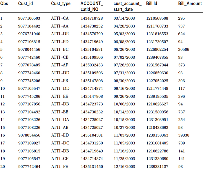
Table 4-15 lists the result of this code.
Table 4-15. Output of proc sort on bill Data Set, Sorted on Bill Amount in Ascending Order
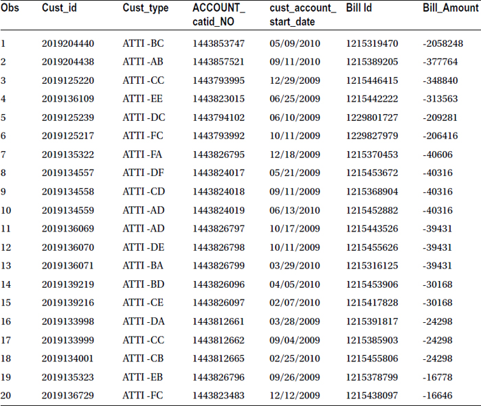
You got the output, and the new table is sorted on bill amount, but the final output has a small surprise for you. The data is sorted in ascending order. Yes! By default SAS sorts data in ascending order. If you want to sort the data, you need to give the descending option. In this example, you want to see the top ten bill payers. Also note that the negative numbers might indicate that the customers have paid more than their billed amount in previous cycles. The following code sorts the table in descending order of bill amount:
proc sort data=MYDATA.bill out=mydata.bill_top;
by descending Bill_Amount ;
run;
proc print data=mydata.bill_top (obs=20);
run;
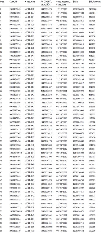
Table 4-16 lists the output.
Table 4-16. Output of proc sort on bill Data Set, Sorted on Bill Amount Descending Order
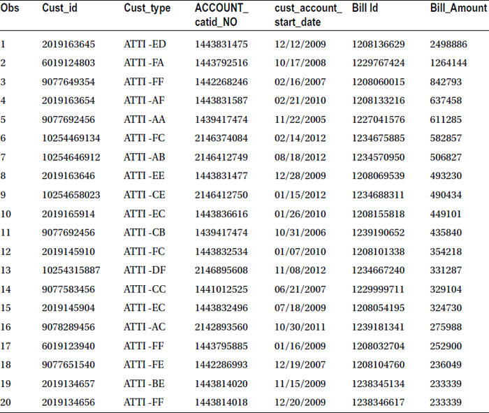
Now Table 4-16 clearly shows the top ten bill payers. Let’s proceed from here.
Using the same example, imagine that you want to first sort the customers based on their account start date old to new, and if there are any ties, then you want to sort them based on bill amount. Here is the SAS code to do that:
proc sort data=MYDATA.bill out=mydata.StartDate_bill_top;
by cust_account_start_date descending  Bill_Amount ;
run;
proc print data=mydata.StartDate_bill_top(obs=20);
run;
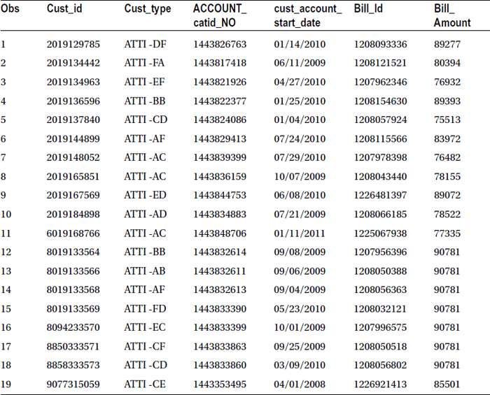
Table 4-17 lists the output.
Table 4-17. Output of proc sort on Bill Data Set, Sorted on Account Start Date and Bill Amount
The data in Table 4-17 is sorted based on account start date in ascending order and bill amount in descending order.
PROC SORT Along with Other Options
You can rename, keep, drop, and use a where condition in a proc sort procedure. The following example sorts the data based on bill amount and keeps only the accounts where the bill is more than 100,000.
proc sort data=MYDATA.bill out=mydata.bill_top100k;
by descending Bill_Amount ;
where Bill_Amount>100000;
run;

proc print data=mydata.bill_top100k;
run;
Table 4-18 lists the output.
Table 4-18. Output of proc sort with where Clause on the Bill Data Set (Bill_Amount>100000)
PROC SORT for Removing Duplicates
Apart from simply sorting the data, proc sort can also be used for removing duplicate records. There are several occasions where you want to remove the duplicates. Imagine salary records of a set of employees. In any case, you don’t want to credit salary more than once for any single employee. Using proc sort, you can very well remove the duplicate records. You use the nodup option in the proc sort code to remove the duplicate records.
Just as an example, you want to sort some data based on customer ID and remove the duplicate records in the same step. The following code sorts the whole data based on customer ID and also removes the duplicates from the input data before storing it in a new data set:
proc sort data=MYDATA.bill out=mydata.bill_wod nodup;
by cust_id   ;
run;
Here is the log message from SAS:
NOTE: There were 31183 observations read from the data set MYDATA.BILL.
NOTE: 19 duplicate observations were deleted.
NOTE: The data set MYDATA.BILL_WOD has 31164 observations and 6 variables.
NOTE: PROCEDURE SORT used (Total process time):
      real time           0.06 seconds
      cpu time            0.05 seconds
The log message clearly states that there are 19 duplicate observations and they are deleted.
You can see the preceding code removes the duplicate records. When a complete observation is repeated, then it will be removed using the nodup option. What if you want to remove the records based on a few variables? For example, say you want to remove all the repetitions based on bill ID. Every bill should have one ID, and it should not be repeated. In this case, the nodup option is not sufficient. You have to use the nodupkey so that the duplicates will be deleted based on the key, in other words, the bill ID.
This code removes the duplicates based on bill ID:
proc sort data=MYDATA.bill out=mydata.bill_cust_wod nodupkey;
by Bill_Id ;
run;
Here is the log message from SAS:
NOTE: There were 31183 observations read from the data set MYDATA.BILL.
NOTE: 93 observations with duplicate key values were deleted.
NOTE: The data set MYDATA.BILL_CUST_WOD has 31090 observations and 6 variables.
NOTE: PROCEDURE SORT used (Total process time):
      real time           0.03 seconds
      cpu time            0.04 seconds
There are 93 entries in the bill data set with repeated bill IDs. They might have different bill values. Also, they may be of different account types, but the bill ID is still the same. Hence, they will be deleted.
Taking Duplicates into a New File
In the previous section, you saw how to remove duplicates. Many times you will want to put all these duplicate entries into a different file and use them in further analysis. The out option gives you the output file but not the duplicates. You need to use the dupout option to put the duplicates into a separate file.
The following code sends the duplicate entries into a new file. This code is using the same example as in the earlier section.
proc sort data=MYDATA.bill out=mydata.bill_wod nodup dupout=mydata.nodup_cust_id  ;
by cust_id   ;
run;
proc print data=mydata.nodup_cust_id;
run;
Table 4-19 lists the output of this code.
Table 4-19. Duplicate cust_id Records of the Bill Data Set Put into a Separate File
Now you repeat the same process for Bill_id and put the duplicate records into a separate file.
proc sort data=MYDATA.bill out=mydata.bill_cust_wod nodupkey dpout=mydata.nodupkeys_bill_id ;
by Bill_Id ;
run;
proc print data=mydata.nodupkeys_bill_id;
run;
Table 4-20 lists the output of this code.
Table 4-20. Duplicate bill_id Records of the Bill Data Set Taken into a Separate File
In this section, you will plot the data using SAS. SAS can produce most of the graphs that are used in day-to-day business. You use the GPLOT and GCHART procedures for drawing the graphs.
Using the gplot and Gchart procedures, you can draw one variable and two variable graphs. For example, you want to draw a graph that shows the relation between budget and reach. As the market campaign budget increases, what happens to reach? Does it increase unconditionally? You can infer information about these points looking at the scatter plot between budget and reach.
The generic code for drawing a scatter plot follows:
proc gplot data= <data set>;
plot y*x;
run;
Table 4-21 explains this code.
Table 4-21. Code Listing for proc gplot Generic Code
|
Code |
Explanation |
|---|---|
|
proc gplot |
Calling gplot procedure |
|
data=<data set>; |
Data set name |
|
plot y*x; |
Scatter plot between Y and X |
Here is the code for drawing a scatter plot between budget and reach:
symbol i=none;
proc gplot data= market_asset;
plot reach*budget;
run;
Figure 4-1 shows the results from this code.
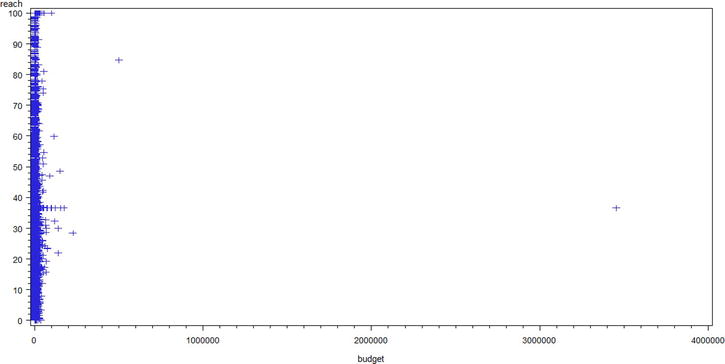
Figure 4-1. A scatter plot for reach versus budget (market_asset data set)
There is no clear conclusion that can be drawn from Figure 4-1. There are few extremely high values in the budget. Let’s draw a scatter plot for a subset.
proc gplot data= market_asset;
plot reach*budget;
where budget  < 100000;
run;
Figure 4-2 shows the results from this code.
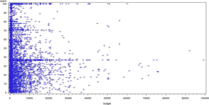
Figure 4-2. A scatter plot for reach versus budget (market_asset data set, budget< 100000)
Here also you can’t see any clear evidence. It doesn’t tell anything; if budget increases, what happens to reach?
Let’s try with an even smaller subset of budget.
proc gplot data= market_asset;
plot reach*budget;
where budget  < 1000;
run;
Figure 4-3 shows the results from this code.
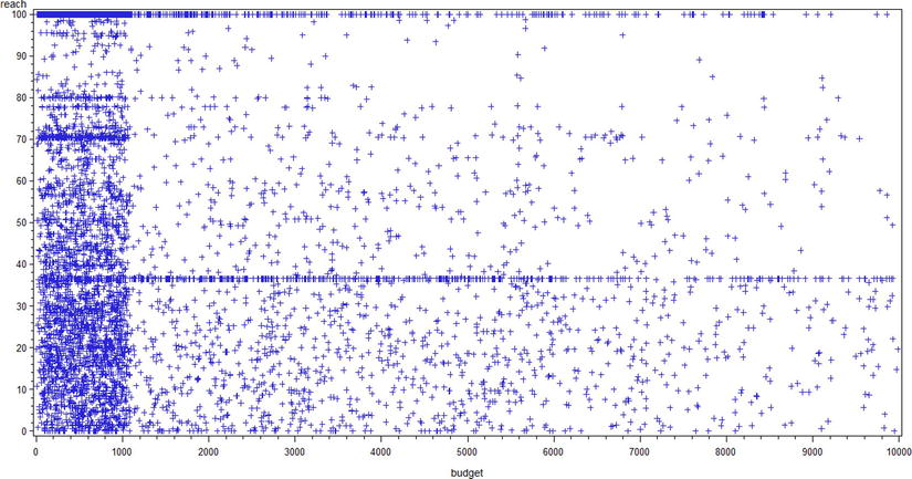
Figure 4-3. A scatter plot for reach versus budget (market_asset data set, budget< 1000)
Again, there is no clear trend on reach versus budget. So, you may conclude that budget and reach are not dependent on each other as far as this input data is concerned.
Bar Chart and Pie Chart Using SAS
You can also plot bar charts using SAS. For this you need to use proc Gchart. To explain this, you’ll again use the same market campaign example. This time you want to see the number of market campaigns in each category. Here is the code:
proc gchart data= market_asset;
vbar category;
Run;
Figure 4-4 shows the output of this code.
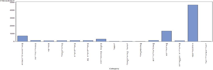
Figure 4-4. Category-wise number market campaigns: a bar chart using proc gchart
Similarly, you can create a pie chart on the same data using the following code:
proc gchart data= market_asset;
pie category ;
Run;
Figure 4-5 shows the output of this code.

Figure 4-5. Category-wise number market campaigns: a pie chart using proc gchart
You can draw the same bar and pie charts in three dimensions (3D) using the following code. See Figures 4-6 and 4-7.
/* 3D bar chart */

proc gchart data= market_asset;
vbar3d category ;
Run;

/* 3D pie chart */

proc gchart data= market_asset;
pie3d category ;
Run;

Figure 4-6. Category-wise number market campaigns: a 3D bar chart using proc gchart
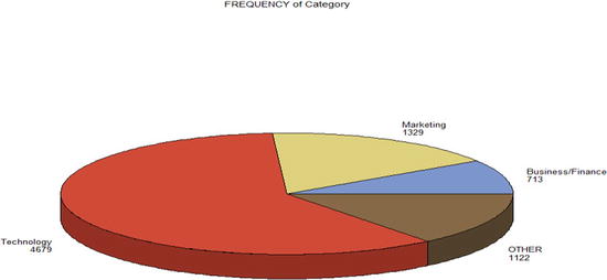
Figure 4-7. Category-wise number market campaigns: a 3D pie chart using proc gchart
The PROC SQL procedure is a boon for those who are coming from a database and SQL background. SAS has a SQL engine, and you can turn it on by using PROC SQL. Once you use a PROC SQL statement in the code, then you can write the standard SQL commands to handle data. You need to finally use a QUIT statement to stop the SQL engine. A generic template for the code follows:
proc sql;

<SQL Statements> ;

Quit;
Note that you use QUIT instead of a usual RUN statement in proc sql. This is just to stop the execution of SQL statements. If you don’t use QUIT, the SQL engine runs until you explicitly terminate it.
PROC SQL Example 1
You will use the same familiar market campaign data again. The manager of this market campaign analysis wants to see only campaigns that are in the business and finance categories. First you write some SQL code in SAS to take the required subset of the data and to put it into a new data set. The code is pretty straightforward.
proc sql;
create buss_fin /* This is the new dataset */
as select *
from  market_asset
where Category= 'Business/Finance';
Quit;
Here is the log file message for the preceding code:
87   proc sql;
88   create table buss_fin
89   as select *
90   from  market_asset
91   where Category= 'Business/Finance';
NOTE: Table WORK.BUSS_FIN created, with 713 rows and 7 columns.

92   Quit;
NOTE: PROCEDURE SQL used (Total process time):
      real time           0.01 seconds
      cpu time            0.01 seconds
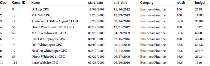
There are 713 rows in the new data set. Let’s print the first ten observations just to have a feel of the data.
proc print data=buss_fin(obs=10);
run;
Table 4-22 lists the output of the code.
Table 4-22. A Snapshot of the buss_fin Data Set
PROC SQL Example 2
If the manager wants to see the total budget spend in each category, the following SQL code can be used:
proc sql;
select  Category, sum(budget) as total_budget
from  market_asset
group by  Category;
Quit;
Table 4-23 lists the output of this code.
Table 4-23. Category-wise Budget Spends in the Market Campaign Data
|
Category |
total_budget |
|---|---|
|
Business/Finance |
5388826 |
|
Construction |
174274.5 |
|
Energy |
66633 |
|
Government |
124867 |
|
Healthcare |
522192 |
|
Healthcare UK |
692567 |
|
Human Resources |
1288243 |
|
Legal |
18624.5 |
|
Local Government |
32442 |
|
Management |
5102 |
|
Manufacturing |
194594 |
|
Marketing |
4920834 |
|
Retail/e-commerce |
235812.9 |
|
Technology |
20757224 |
|
testingvertical |
1234 |
![]() Note The SQL code used for left, right, and inner joins remains the same in proc sql. It’s not repeated here. You may want to refer to any standard SQL text or Google it. Google search strings like left join in SAS should give you the required answer.
Note The SQL code used for left, right, and inner joins remains the same in proc sql. It’s not repeated here. You may want to refer to any standard SQL text or Google it. Google search strings like left join in SAS should give you the required answer.
Analysts might have to work with multiple data sets and join or merge them to prepare one final data set for analysis. Imagine a scenario in the market campaign data. The information on leads is in a different table. You may want to merge these two data sets to prepare a final data set for analysis.
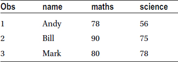
Let’s try to understand these concepts using examples, which has been the usual approach throughout this book. The following code uses two sets of students. Each set has five students. The first set of students has mathematics as a subject in the exam, and the second set has science. The first three students appear in both the data sets. You will consider these two simple data sets to understand the concept of various types of data merging:
data students1;
input name $ maths;
cards;
Andy 78
Bill 90
Mark 80
Jeff 75
John 60
;
data students2;
input name $ science;
cards;
Andy 56
Bill 75
Mark 78
Fred 86
Alex 77
;
Appending is simply affixing the second data set after the first data set. It’s not really a big deal. In the resultant data set, the rows in the second data set will simply appear after the first data set. Here is the code for appending the data sets. You simply use a SET statement.
Data Students_1_2;
set students1 students2;
run;
Here is the log file when you execute this code:
NOTE: There were 5 observations read from the data set WORK.STUDENTS1.
NOTE: There were 5 observations read from the data set WORK.STUDENTS2.
NOTE: The data set WORK.STUDENTS_1_2 has 10 observations and 3 variables.
NOTE: DATA statement used (Total process time):
      real time           0.03 seconds
      cpu time            0.01 seconds
Let’s take a snapshot of the resultant data set (Table 4-24).
proc print data=Students_1_2;
run;
Table 4-24. A Snapshot of the Resultant Students_1_2 Data Set, Using the SET Keyword
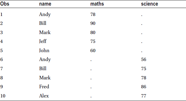
If there are some common columns in the data sets, then they will be populated (as a single column) in the new data set; otherwise, the columns will be left blank. In this data set, the name column is populated automatically, but the mathematics and science columns are left blank in the data rows, which are not applicable.
Table 4-24 shows that Andy, Bill, and Mark are repeated twice each. You see that the SET statement simply appends the data. You may want to do more than that. The SET statement doesn’t work if you want to see both science and math marks against Andy, Bill, and Mark, without repeating their names (Table 4-25). For this, you need to use the MERGE option instead of SET.
Table 4-25. Data Sets with SET and MERGE Options in SAS Code

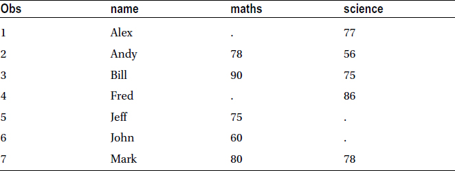
To get the result shown on the right side of Table 4-25, you need to replace set with a merge statement in your SAS code. Sorting is necessary before merging data sets; otherwise, SAS will throw an error. The following is the code for merging two students’ data sets:
proc sort data=students1;
by name;
run;
proc sort data=students2;
by name;
run;

data studentmerge;
Merge students1 students2;
by name;
run;

proc print data=studentmerge;
run;
The log file after execution looks like this:
182  proc sort data=students1;
183  by name;
184  run;

NOTE: There were 5 observations read from the data set WORK.STUDENTS1.
NOTE: The data set WORK.STUDENTS1 has 5 observations and 2 variables.
NOTE: PROCEDURE SORT used (Total process time):
      real time           0.03 seconds
      cpu time            0.03 seconds

185  proc sort data=students2;
186  by name;
187  run;

NOTE: There were 5 observations read from the data set WORK.STUDENTS2.
NOTE: The data set WORK.STUDENTS2 has 5 observations and 2 variables.
NOTE: PROCEDURE SORT used (Total process time):
      real time           0.03 seconds
      cpu time            0.01 seconds

188
189  data studentmerge;
190  Merge students1 students2;
191  by name;
192  run;

NOTE: There were 5 observations read from the data set WORK.STUDENTS1.
NOTE: There were 5 observations read from the data set WORK.STUDENTS2.
NOTE: The data set WORK.STUDENTMERGE has 7 observations and 3 variables.
NOTE: DATA statement used (Total process time):
      real time           0.03 seconds
      cpu time            0.03 seconds
Table 4-26 lists the output.
Table 4-26. A Snapshot of the Resultant studentmerge Data Set, Using the MERGE Keyword
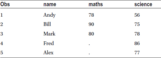
Sometimes the situation demands that you have all the observations from one data set and just the matching observations from the other. In other words, you want to have all the observations from data set 2 and only matching values from data set 1.
Table 4-27 shows the example for data set 1 with the math entries completely filled in and some values blank in the science marks column.
Table 4-27. Example Data Set 1 with Two Blanks in the Science Column
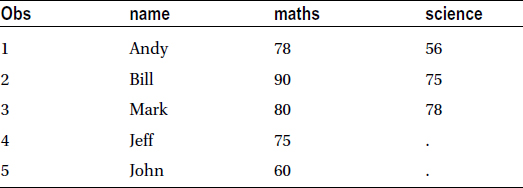
Table 4-28 shows the example for data set 2 with some math entries blank.
Table 4-28. Example Data Set 2 with Two Blanks in the maths Column
At first you get all observations from data set 1 and only the matching observations from data set 2. Here is the code:
data final;
Merge data1(in=a) data2(in=b);
by var;
if a;
run;
The if a statement will keep all the entries from data set 1 and only the matching records from data set 2. Similarly, you can do the reverse by using the following code:
data final1;
Merge data1(in=a) data2(in=b);
by var;
if b;
run;
The if b statement will keep all the entries of data set 2 and keep only the matching records from data set 1.
If you want to keep the records, which appear in both the data sets, you can use an if a and b statement, as given here:
data final2;
Merge data1(in=a) data2(in=b);
by var;
if a and b;
run;
As an exercise, you may want to print the data sets final, final1, and final2 to validate the results.
Matched Merging
To demonstrate the concepts of matched merging in this section, you use the students1 and students2 data sets from the data merging section. You may recall that both had only two columns. The following is the code to keep all records from students1, along with matching records from students2:
/*matched merging example-1 */

proc sort data=students1;
by name;
run;
proc sort data=students2;
by name;
run;

data studentmerge1;
Merge students1(in=a) students2(in=b);
by name;
if a;
run;
Here is the log file for the preceding code:
NOTE: There were 5 observations read from the data set WORK.STUDENTS1.
NOTE: There were 5 observations read from the data set WORK.STUDENTS2.
NOTE: The data set WORK.STUDENTMERGE1 has 5 observations and 3 variables.
NOTE: DATA statement used (Total process time):
      real time           0.03 seconds
      cpu time            0.01 seconds
Table 4-29 is the result of this code.
Table 4-29. Matched Merging Example 1
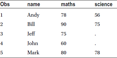
The following code keeps all records from students2, along with matching records in students1:
/*Matched merging example-2 */

data studentmerge3;
Merge students1(in=a) students2(in=b);
by name;
if a and b;
run;
Here is the log file for the preceding code:
NOTE: There were 5 observations read from the data set WORK.STUDENTS1.
NOTE: There were 5 observations read from the data set WORK.STUDENTS2.
NOTE: The data set WORK.STUDENTMERGE2 has 5 observations and 3 variables.
NOTE: DATA statement used (Total process time):
      real time           0.03 seconds
      cpu time            0.01 seconds
Table 4-30 shows the output of this code.
Table 4-30. Matched Merging Example 2
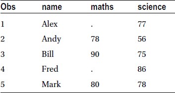
The following code keeps all matching records in students1 and students2:
/* Matched merging example-3 */

data studentmerge3;
Merge students1(in=a) students2(in=b);
by name;
if a and b;
run;
The log file shows the following:
NOTE: There were 5 observations read from the data set WORK.STUDENTS1.
NOTE: There were 5 observations read from the data set WORK.STUDENTS2.
NOTE: The data set WORK.STUDENTMERGE3 has 3 observations and 3 variables.
NOTE: DATA statement used (Total process time):
      real time           0.03 seconds
      cpu time            0.03 seconds
Table 4-31 is the output of this code.
Table 4-31. Matched Merging Example 3
Matched Merging: A Brief Case Study
You have two data sets from a telecom case study: bill data and complaints data. The billing data contains customer- and billing-related variables, whereas complaints data contains the type of complaints given by the customers for the period of the last six months. The complaints data also includes details of the disconnected customers, which are not part of the billing data. You want to do the following to prepare the data for further analysis:
- Sort the billing data by customer ID and remove the duplicates.
- Create a consolidated data set that contains only the existing billing customers who gave complaints. You will also attach the type of comment in the resultant data set; name this data set as active_complaints data.
- Attach the billing details of customers to those who made a complaint. You may want to use it for analyzing the complaints and usage information together.
- Attach the complaints details of customers to those who are actively paying the bill. You may want to use it to get the usage pattern along with the type of complains.
Here is the code and the results for executing these tasks:
- Sort the billing data by customer ID and remove the duplicates.
proc sort data= bill nodupkey;
by cust_id;
run;
The log file shows the following:
NOTE: There were 31183 observations read from the data set WORK.BILL.
NOTE: 13259 observations with duplicate key values were deleted.
NOTE: The data set WORK.BILL has 17924 observations and 6 variables.
NOTE: PROCEDURE SORT used (Total process time):
      real time           0.06 seconds
      cpu time            0.03 seconds
As an exercise, you may want to print a snapshot of the resultant data set.
- Create a consolidated data set that contains only the existing billing customers who made a complaint. Attach the type of comment in the resultant data set. Name the resultant data set active_complaints.
proc sort data=    bill nodupkey;
by cust_id;
run;

proc sort data=    complaints nodupkey;
by cust_id;
run;

data  active_complaints;
merge  bill(in=a)  complaints(in=b);
by     cust_id;
if a and b;
run;

proc print data= active_complaints(obs=10) noobs;
run;
The following is the log file for the previous code:
NOTE: There were 17924 observations read from the data set WORK.BILL.
NOTE: There were 29687 observations read from the data set WORK.COMPLAINTS.
NOTE: The data set WORK.ACTIVE_COMPLAINTS has 12638 observations and 11 variables.
NOTE: DATA statement used (Total process time):
      real time           0.03 seconds
      cpu time            0.03 seconds
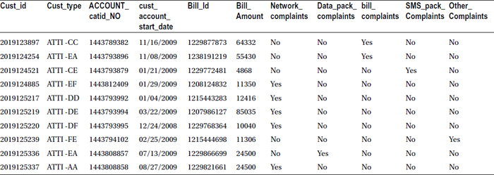
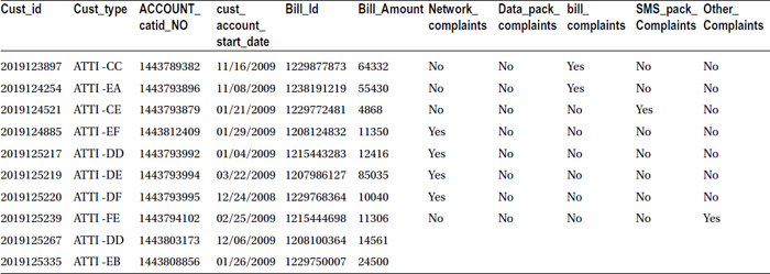
Table 4-32 lists the output snapshot of this code set.
Table 4-32. Consolidated Data Set That Contains Only the Existing Billing Customers Who Gave Complaints
- Attach the billing details of customers to the customers who made complaints.
data  complaints_bill;
merge  bill(in=a)  complaints(in=b);
by     cust_id;
if b;
run;

proc print data= complaints_bill(obs=10) noobs;
run;
The log file message for this code is as follows:
NOTE: There were 17924 observations read from the data set WORK.BILL.
NOTE: There were 29687 observations read from the data set WORK.COMPLAINTS.
NOTE: The data set WORK.COMPLAINTS_BILL has 29687 observations and 11 variables.
NOTE: DATA statement used (Total process time):
      real time           0.10 seconds
      cpu time            0.11 seconds
Table 4-33 shows the output snapshot resulting from this code.
Table 4-33. Billing Details of Customers to the Customers Who Gave Complaints
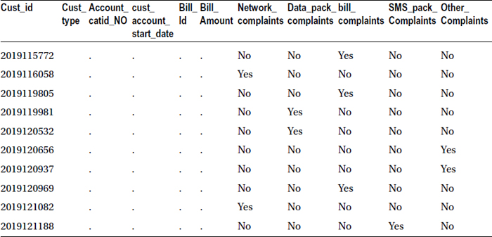
It looks like the first ten observations don’t have any bill details. So, let’s sort the resultant data set based on the bill amount.
proc sort data= complaints_bill;
by descending Bill_Amount;
run;

proc print data= complaints_bill(obs=10) noobs;
run;
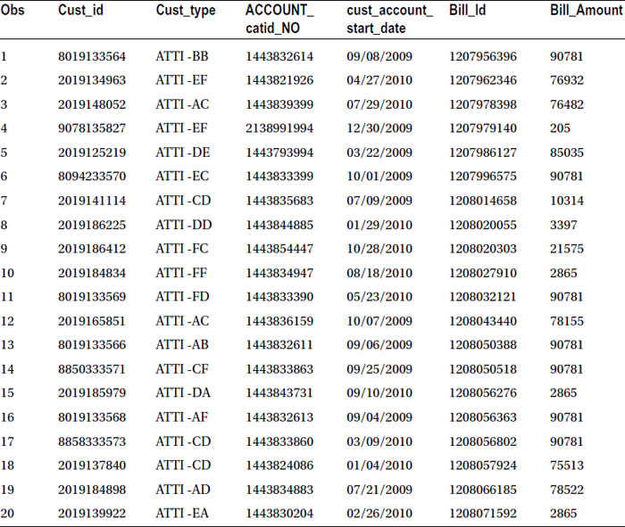
Table 4-34 shows the snapshot of output when this code is executed.
Table 4-34. Output of proc sort on complaints_bill with Descending Order of Bill Amount
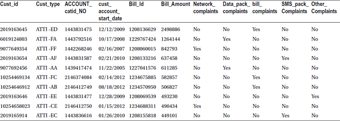
The sorted output in Table 4-34 makes sense now.
- Attach the complaints details of customers to the customers who are actively paying bill.
data  bill_with_complaints;
merge  bill(in=a)  complaints(in=b);
by     cust_id;
if a;
run;

proc print data= bill_with_complaints(obs=10) noobs;
run;
The log file when this code is executed is as follows:
NOTE: There were 17924 observations read from the data set WORK.BILL.
NOTE: There were 29687 observations read from the data set WORK.COMPLAINTS.
NOTE: The data set WORK.BILL_WITH_COMPLAINTS has 17924 observations and 11 variables.
NOTE: DATA statement used (Total process time):
      real time           0.10 seconds
      cpu time            0.07 seconds
Table 4-35 lists the output snapshot.
Table 4-35. Complaints Details of Customers to the Customers Who Are Actively Paying Bill
Conclusion
In this chapter, you learned some commonly used SAS functions and procedures along with options, which make them more useful for analysis. The chapter also discussed creating charts and data merging using SAS. In addition, you learned about the basics of analytics and basic programming in SAS, which is undoubtedly the most widely used analytical tool under the sun.
Next, in Chapter 5, you will enter the world of business analytics and use the concepts you have learned so far. You will learn more programming and analysis concepts. You are going to learn about basic descriptive statistics, correlation, and predictive modeling in coming chapters. The SAS knowledge gained in the past few chapters is vital in executing the analytics algorithms in the coming chapters. Good luck! And get ready for more fun and excitement.