
![]()
Data Exploration, Validation, and Data Sanitization
Preparing the data for the actual analysis is an important portion of any analytics project. The raw data comes from a variety of sources such as classical relational databases, flat files, spreadsheets, and unstructured data from sources such as social media text. A project may contain both structured and unstructured data, and to add to the complexity, there can be numerous data sources. As you would expect, the data will have a lot of challenges—both in quality and in quantity. An analyst needs to first read the data from its sources, which itself can be a challenging task, and then parse it to be useful for any further analysis. SAS needs data to be in its own datasets before you can use any of its routines for analysis. In short, the raw data is not always ready for the analysis; it needs to be validated and cleaned before the analysis.
Considering the importance of the topic, we have treated this topic in sufficient detail. This chapter first makes you aware of the general issues that you may face while preparing data for analysis. We then cover the topics of data validation and cleaning. Finally, we take a very detailed case study in the banking domain to demonstrate the concepts with actual data.
Data Exploration Steps in a Statistical Data Analysis Life Cycle
The previous chapters dealt with applications of basic descriptive statistics. It has already been established that data analysis can yield great results if used effectively. Figure 7-1 recaps the steps followed in statistical data analysis.

Figure 7-1. Steps in the data analysis project
Once the data business objectives have been established, a complete understanding of the data is necessary before proceeding with the analysis process. The data preparation step in the second column in the order, shown in Figure 7-1, raises the following questions:
- Why is understanding and exploring data such an important step in statistical analysis?
- Why does this step need to be mentioned along with other important steps such as descriptive analysis and predictive modeling?
The following example will address these two questions.
Example: Contact Center Call Volumes
Consider the call volume data for a typical customer contact center of a large organization. The data snapshot in Table 7-1 has just three columns. The first column is the day, the second column is the hour of the day, and the third column is the call volume (number of calls) in a given hour. The data is recorded for five consecutive days.
Table 7-1. Call Volume Data
|
Day |
Hour |
Volume |
|---|---|---|
|
1 |
1 |
3,504 |
|
1 |
2 |
3,378 |
|
1 |
3 |
6,872 |
|
1 |
4 |
5,993 |
|
1 |
5 |
3,093 |
|
1 |
6 |
3,512 |
|
1 |
7 |
4,142 |
|
1 |
8 |
6,441 |
|
1 |
9 |
61,906 |
|
1 |
10 |
43,175 |
|
1 |
11 |
49,989 |
|
1 |
12 |
9,862 |
|
1 |
13 |
18,231 |
|
1 |
14 |
46,282 |
|
1 |
15 |
36,665 |
Say you are trying to answer the following: What is the average number of calls? Is it true that the average number of calls in the first 8 hours tends to be less than rest of the 16 hours? The following SAS code needs to be commissioned to do this:
/*Import the data set into SAS */
PROC IMPORT OUT = WORK.call_volume
DATAFILE= "D:BackupSkyDriveBooksContentChapter-12 Data
Exploration and CleaningData setsCall_volume.csv"
DBMS=CSV REPLACE;
     GETNAMES=YES;
     DATAROW=2;
RUN;

/*Get the contents of the SAS data set */
Proc contents data=WORK.call_volume varnum;
run;
The varnum option in the preceding code lists the variables in the order in which they appear in the original data set. SAS usually prints the variables based on alphabetical order.
Refer to Table 7-2 for the output of this code.
Table 7-2. The Variable List from SAS Output For PROC CONTENTS

The PROC MEANS needs to be executed in order to find the average values of the call volume per hour.
The following SAS code finds out the mean on the variable call_volume.

Title'Overall mean of the call volume';
Proc means data=WORK.call_volume ;
var volume ;
run;
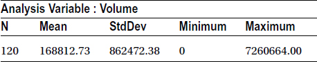
Proc means data gives the output in Table 7-3 by default.
Table 7-3. Output Of PROC MEANS On call_volume Data set
Since you require only the mean, you can use the mean option in the code, as follows:
Title'Overall mean of the call volume';
proc means data=WORK.call_volume mean;
var volume ;
run;
Table 7-4 shows the output of the preceding code.
Table 7-4. The Mean for Variable volume
|
Mean |
|---|
|
168,812.73 |
Following is the code to find the mean call volume for the first eight hours.
Title 'Mean of the call volume in 1 to 8 Hours';
proc means data=WORK.call_volume mean;
var volume;
where Hour <9;
run;
Table 7-5 shows the output of the preceding code.
Table 7-5. Mean of the Call Volume in Hours 1 to 8
|
Mean |
|---|
|
417,169.30 |
Following is the code to find the mean call volume for the later 16 hours, that is, mean call volume between 9 to 24 hours.
Title 'Mean of the call volume in 9 to 24 Hours';
procmeans data=WORK.call_volume mean;
var volume;
where  Hour ge 9;
run;
title;
Table 7-6 shows the output of the preceding code.
Table 7-6. Mean of the Call Volume in Hours 9 to 24
|
Mean |
|---|
|
44,634.44 |
The overall mean of all call numbers across the file was calculated in the SAS code preceding Table 7-4. The same mean for the first 8 hours and the same data for the subsequent 16 hours were then calculated (Tables 7-5 and 7-6). So, a simple proc means the SAS script helps find that the overall average number of calls per hour is 168,812. The assumption that the average number of calls per hour in the first 8 hours is less than the rest of 16 hours is not true. The call rate in the first 8 hours is almost 10 times higher than the next 16 hours of data.
The contact center can now deploy resources based on the average number of calls per hour. However, the manager reviews these results and rejects them.
The rationale behind the rejection is given next.
Need for Data Exploration and Validation
To explain the need for data exploration and validation, we will continue by extending the same contact center call volumes example.
- The manager knows by experience that the average number of calls per hour is generally between 50,000 to 100,000.
- He also questions the likelihood of there being more calls during the first 8 hours of the day (12 a.m. to 8 a.m.) compared to the next 16 hours. His experience also tells him that the call rate should be considerably higher in the later 16 hours.
His confidence necessitates a reexamination of the results from the raw call volume data for all five days.
Table 7-7 lists the data for the number of calls every hour, for 24 hours each day, for 5 days. Each data row contains the observation number, the hour, and the number of calls received in that hour.
Table 7-7. Hourly Call Volume Data for 5 Days


Note that there are a few unusually high values in the Volume column on day 3. They may be true entries, but the high call rates might be because of some incidents that do not occur every day. The other entries look to be in order. Also, note that the value for the 17th hour is zero on days 2, 3, and 4. These zeros might be because of technical mistakes or any other unknown reason. These rarely occurring values are the outliers. You need to remove them and calculate the same three averages again. Restrict the sample to the call volumes between 1,000 and 100,000 for doing so.
/* Call volume subset */
Data call_Volume_subset;
Set WORK.call_volume;
if volume >1000 and volume<100000;
run;
When the preceding SAS code is executed, the log file shows the following:
NOTE: There were 120 observations read from the data set WORK.CALL_VOLUME.
NOTE: The data set WORK.CALL_VOLUME_SUBSET has 113 observations and 3 variables.
NOTE: DATA statement used (Total process time):
real time           0.01 seconds
cpu time            0.01 seconds
The new average values are as follows:
Title 'Overall mean of the call volume';
proc means data=WORK. call_Volume_subset mean;
var volume ;
run;
Table 7-8 shows the output of the preceding code.
Table 7-8. Overall Mean of call_volume
|
Mean |
|---|
|
32,952.86 |
The following code is for calculating the mean of the first 8 hours, after removing the outliers.
Title 'Mean of the call volume in 1 to 8 Hours';
proc means data=WORK. call_Volume_subset mean;
var volume;
where Hour <9;
run;
Table 7-9 shows the output of the preceding code.
Table 7-9. Mean of the Call Volume in 1 to 8 Hours
|
Mean |
|---|
|
4,247.72 |
The following code is for calculating the mean of the later 16 hours, after removing the outliers.
Title 'Mean of the call volume in 9 to 24 Hours';
proc means data=WORK. call_Volume_subset mean;
var volume;
where  Hour ge 9;
run;
title;
Table 7-10 shows output of the preceding code.
Table 7-10. Mean of the Call Volume in Hours 9 to 24
|
Mean |
|---|
|
46,373.44 |
The modified data set indicates that the average number of calls per hour is 32,952. The number of calls in the first 8 hours is almost 10 times less than the remaining 16 hours. These numbers make business sense and are in accordance with the manager’s experience. The analytics inferences need not always match the experience. When analyzed, the opposite may be true. Whatever the case, the analytics results should always be rational and make business sense. The blind averages in the call center example on the raw data resulted in the opposite of what the business was experiencing. The careful examination of data revealed the presence of outliers.
Although 7 out of 120 records were troublesome, the results had large differences. It is always a good idea to inspect data routinely before starting the analysis.
Issues with the Real-World Data and How to Solve Them
Real-world data is often crude and cannot be analyzed in its given form. The following are some of the frequent challenges encountered in data made available for analytics projects:
- Real-world data often contains missing values, which may be the data points where data is not captured or is not available.
- The data sets often contain outliers. For example, the monthly income of a few selected individuals in a sample is recorded in millions.
- A few fields in some data sets are sometimes constant, such as seeing age = 11 and number of personal loans = 6 in all the records.
- The data is simply erroneous, such as number of dependents = –3.
- The data may contain default values such as 999999, 1111111, #VALUE, NULL, or N/A.
- The data is incomplete or is not available at the transaction level but only at the aggregate level, such as most economic indicators. If you are performing analysis at the transaction level, then you may incur a lot of error.
- The data is insufficient. The vital variables required for analysis may not be present in the data set.
Missing Values
Missing values and the outliers are the two most common issues in data sets. The nonavailability of data is also a frequent issue. Sometimes a considerable size of the population or sample might have missing values. The following are a couple of examples:
- There might be a lot of missing values in the credit bureau data related to developing and underdeveloped countries.
- A marketing survey with optional fields will definitely have missing values by design.
The Outliers
The outliers are not exactly errors, but they can be the cause for misleading results. An outlier is typically a value that is very different from the other values of that variable. An example is when, in a given data column, 95 percent of the data is between certain limits but the rest of the 5 percent is completely different, which may significantly change the overall results. This issue occurred with the call volumes example. A couple of other examples of outliers are as follows:
- Insurance claim data, where just 2 percent of claims are more than $5 million and the rest are less than $800,000
- Superstore data on customer spend, where in a month just 4 customers spend $50,000 and the rest of the customers spend less than $6,000
These are just two examples of the issues that may be present in the raw data that is made available for analysis. There may be several other issues at the data set level, such as format-related challenges with variable types such as dates, numbers, and characters. The variable lengths may not make business sense. In addition, several other data issues might arise while transferring the data from one database platform to other. This chapter concentrates only on the data analysis–related issues.
Manual Inspection of the Dataset Is Not a Practical Solution
The small amount of data in the call volume example made it possible to manually look for abnormalities in the data. This is not possible with larger data sets with many variables. A data set with more than 100 variables and 1 million records does not allow for it to be examined manually for the outliers and other data-related issues.
Therefore, you need a sound, scientific method to look at the data before the analysis. The data exploration process should highlight all the hidden problems that are hard to identify manually.
Removing Records Is Not Always the Right Way
Can the troubled records simply be removed? Is that the right way? If not, what is the best possible way to deal with data errors? After identifying issues such as outliers and missing values, it is tempting to drop these erroneous records and proceed with the rest of the analysis. But doing so also gets rid of some precious information.
For example, consider the employee profile data given in Table 7-11. The data is divided into seven columns:
- EmpID: Employee ID
- Name: Name of the employee
- Age: Age of the employee
- Qualification: Educational qualification of the employee
- Experience: Years of experience of employee
- Gender: Gender of the employee
- Team: The team in which the employee is working
Table 7-11. Employee Profile Data
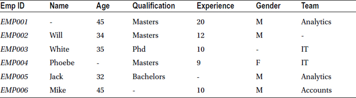
It’s apparent from the columns that every record has at least one field missing, and hence dropping records with missing values is not a solution. You need a robust and consistent solution.
Understanding and Preparing the Data
Chapter 6 used the box-plot technique to identify the outliers in a variable. A few simple descriptive statistics techniques and checkpoints can be used in data analysis as well in order to completely understand the data. The data needs to be understood and cleaned first, as discussed in the earlier call volume example. Only then will it be ready for analysis. The following sections examine data exploration, validation, and cleaning in detail.
Data Exploration
The first data inspection step is to get a complete understanding of the data and the minute details of its structure. The following questions need to be answered:
- How is the data structured?
- What are the variables?
- What are their types?
- How many variables are there?
- How many records are there?
- Are there any missing values?
Data Validation
Data validation will answer the following questions:
- Are all the values correct?
- Are there any outliers?
- Are the variable types correct?
- Does the data match the data dictionary, which describes all the variables involved in the data set?
All these questions deal with the accuracy checks on the data. This step can be executed during data exploration or can be carried out as a separate step. Simple descriptive statistics techniques are brought into play at this stage.
Data Cleaning
You can identify almost all the issues with the data set using data exploration and data validation. Next, the data needs to be cleaned and made ready for the analysis. The outliers and missing values along with any other errors need to be fixed by appropriate substitutions. But is the process of data cleaning the same if the variable is discrete or continuous? What if just 1 percent of the values are missing in the data? What if 30 percent of the values are missing? Is the treatment the same for the 10 percent, 30 percent, and 90 percent missing values cases?
The steps of exploring, validating, and cleaning data take a considerable amount of time in the project life cycle, sometimes as high as 70 percent of the total person hours available for the project. There are no shortcuts either. You need to explore all the variables to understand and resolve the issues. The subsequent topics in this chapter will discuss ways of understanding, validating, and cleaning the data using a credit risk case study.
Data Exploration, Validation, and Sanitization Case Study: Credit Risk Data
What follows is a credit risk case study, which we use throughout this chapter to demonstrate various steps and concepts pertaining to data preparation prior to the start of the actual analysis process.
THE CREDIT SCORING SYSTEM
Reference: The data set used in this case study is based on and used with permission from Kaggle’s web site at https://www.kaggle.com/c/GiveMeSomeCredit.
It is common knowledge that banks offer several products, such as personal loans, credit cards, mortgages, and car loans. Every bank seeks to evaluate the risks associated with a customer before issuing a loan or a credit card. Each customer is assessed based on a few crucial parameters, such as the number of previous loans, average income, age, number of dependents, and so on. The banks use advanced analytics methodologies and build predictive models to find the probability of a default before issuing the card or a loan.
Historical customer payments and usage data is used for building a predictive model, which will quantify the risk associated with each customer. The bank decides a cutoff point, and any customer with a higher risk than the cutoff is rejected. This methodology of quantifying the risk is called credit scoring. Each customer gets a credit score as a result of this model, which is built on historical data. The higher the credit score, the better a customer’s probability of availing a credit is. In general, a credit score is between 0 and 1000, but this is not mandatory. For example, if a customer gets a credit score of 850, her application for a loan or credit card may be approved. On the other hand, if a customer scores 350, her probability of getting credit becomes almost zero.
One needs to be careful about data errors such as missing values and outliers while building credit risk models. An error might negate the credibility of the entire model if not handled well, and one major default on a loan may negate the profits earned from 100 good cases. The model has to be robust under all circumstances because no bank wants to give a high score to a bad customer. Hence, data exploration, validation, and cleaning become important in models involving financial transactions.
DATA DICTIONARY
Reference: The base data set is taken from Kaggle and modified.
Given in Tables 7-12 and 7-13 is the data set for building the predictive model. A data dictionary that usually accompanies the data explains all the variable details. Each variable needs to be examined in order to understand, validate, and clean if necessary. The following are the details given by the bank’s data team.
The historical data for 250,000 borrowers, collected over a two-year performance window, is provided. Part of this data is used for building the models, and some data is set aside for testing and validation purposes.
The data set file name is Customer_loan_data.csv, and the data dictionary (the variable details) is given in Table 7-12.
Table 7-12. Data Dictionary for the Example
|
Variable Name |
Description |
Type |
|---|---|---|
|
SeriousDlqin2yrs |
Person experienced 90 days past due delinquency or worse |
Y/N |
|
RevolvingUtilizationOfUnsecuredLines |
Total balance on credit cards and personal lines of credit except real estate and no installment debt such as car loans divided by the sum of credit limits |
Percentage |
|
Age |
Age of borrower in years |
Integer |
|
NumberOfTime30-59DaysPastDueNotWorse |
Number of times borrower has been 30 to 59 days past due but no worse in the last 2 years |
Integer |
|
DebtRatio |
Monthly debt payments, alimony, living costs divided by monthly gross income |
Percentage |
|
MonthlyIncome |
Monthly income |
Real |
|
NumberOfOpenCreditLinesAndLoans |
Number of open loans (installment loans such as a car loan or mortgage) and lines of credit (such as credit cards) |
Integer |
|
NumberOfTimes90DaysLate |
Number of times borrower has been 90 days or more past due |
Integer |
|
NumberRealEstateLoansOrLines |
Number of mortgage and real estate loans including home equity lines of credit |
Integer |
|
NumberOfTime60-89DaysPastDueNotWorse |
Number of times borrower has been 60 to 89 days past due but no worse in the last 2 years |
Integer |
|
NumberOfDependents |
Number of dependents in family excluding themselves (spouse, children, and so on) |
Integer |
All the variables in Table 7-12 are related to credit risk. Table 7-13 provides a detailed explanation of the variables.
Table 7-13. Detailed Explanation of the Variables
|
Variable Name |
Description |
Type |
|---|---|---|
|
SeriousDlqin2yrs |
Person experienced 90 days past due delinquency or worse. These accounts are also known as bad accounts. The bad definition changes from product to product. For example, a serious delinquency for credit cards is 180 days delinquent. This might be a loan or a mortgage, and hence 90 days past due is serious delinquency. In general, this is the target variable that needs to be predicted. |
Y/N |
|
RevolvingUtilizationOfUnsecuredLines |
Total balance on credit cards and personal lines of credit except real estate and number of installment debt such as car loans divided by the sum of credit limits. Consider a credit card with $100,000 as the credit limit. If $25,000 is used on average every month, the utilization percentage is 25 percent. If $10,000 is used on an average, the utilization is 10 percent. So, utilization takes values between 0 and 1 (0 to 100 percent). |
Percentage |
|
Age |
Age of borrower in years. |
Integer |
|
NumberOfTime30-59DaysPastDueNotWorse |
Number of times borrower has been 30 to 59 days past due but no worse in the last 2 years. This data spans 2 years. How many times was a customer 30 days late but not later than 59 days? Once, twice, three, or six times? |
Integer |
|
DebtRatio |
Monthly debt payments, alimony, living costs divided by monthly gross income. Debt to income ratio. With an income of $50,000, debt is $10,000, and debt ratio is 20 percent. Hence, the debt ratio can take any value between 0 and 100 percent. It can also be slightly more than 100 percent. |
Percentage |
|
MonthlyIncome |
Monthly income. |
Real |
|
NumberOfOpenCreditLinesAndLoans |
Number of open loans (an installment loan such as car loan or mortgage) and lines of credit (such as credit cards). |
Integer |
|
NumberOfTimes90DaysLate |
Number of times borrower has been 90 days or more past due. This data is for 2 years. How many times a customer was is 90 days late? Once, twice, three times, or five times? |
Integer |
|
NumberRealEstateLoansOrLines |
Number of mortgage and real estate loans including home equity lines of credit. |
Integer |
|
NumberOfTime60-89DaysPastDueNotWorse |
Number of times borrower has been 60 to 89 days past due but no worse in the last 2 years. This data is for 2 years. How many times was a customer 60 to 89 days late but not worse? Once, twice, three, or five times? |
Integer |
|
NumberOfDependents |
Number of dependents in family excluding applicant (spouse, children, and so on). |
Integer |
The following sections will use simple descriptive statistics techniques to explore, validate, and sanitize the credit risk data.
The following SAS code imports the .csv file into SAS:
/*Import the customer raw data into SAS */
PROCIMPORT OUT= WORK.cust_cred_raw
DATAFILE= "C:UsersGoogle DriveTrainingBooksContentChapter-12 Data Exploration and CleaningDatasetsCustomer_loan_data.csv"
DBMS=CSV REPLACE;
     GETNAMES=YES;
     DATAROW=2;
RUN;
Here are the main notes from the SAS log file of the preceding code, when executed:
NOTE: The infile 'C:UsersGoogle DriveTrainingBooksContentChapter-12 Data
      Exploration and CleaningDatasetsCustomer_loan_data.csv' is:

      Filename=C:UsersGoogle DriveTrainingBooksContentChapter-12 Data Exploration
and CleaningDatasetsCustomer_loan_data.csv,
      RECFM=V,LRECL=32767,File Size (bytes)=14516824,
      Last Modified=05Mar2014:14:55:27,
      Create Time=05Mar2014:12:54:18

NOTE: 251503 records were read from the infile 'C:UsersGoogle
      DriveTrainingBooksContentChapter-12 Data Exploration and
      CleaningDatasetsCustomer_loan_data.csv'.
      The minimum record length was 33.
      The maximum record length was 64.
NOTE: The data set WORK.CUST_CRED_RAW has 251503 observations and 13 variables.
NOTE: DATA statement used (Total process time):
real time           1.82 seconds
cpu time            1.52 seconds

251503 rows created in WORK.CUST_CRED_RAW from C:UsersGoogle
DriveTrainingBooksContentChapter-12 Data Exploration and
CleaningDatasetsCustomer_loan_data.csv.
NOTE: WORK.CUST_CRED_RAW data set was successfully created.
NOTE: PROCEDURE IMPORT used (Total process time):
real time           2.07 seconds
cpu time            1.76 seconds
According to the preceding analysis, there are no major warnings or errors. The name of the SAS data set is cust_cred_raw. The following is the process of data exploration.
Step 1: Data Exploration and Validation Using the PROC CONTENTS
PROC CONTENTS data is used to get basic details about the data, such as the number of records variables and variable types. Because the intention is to understand the data completely without actually opening the data file, PROC CONTENTS can be the starting point to get metadata (data about data) and related details.
The SAS code for contents looks like this:
title'Proc Contents on raw data';

proc contents data= WORK.cust_cred_raw varnum ;
run;
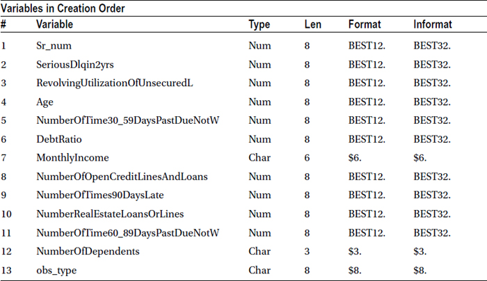
The preceding SAS code generates the output in Table 7-14.
Table 7-14. Output of proc contents on cust_cred_raw Data Set

|
Engine/Host Dependent Information | |
|---|---|
|
Data Set Page Size |
12288 |
|
Number of Data Set Pages |
2150 |
|
First Data Page |
1 |
|
Max Obs per Page |
117 |
|
Obs in First Data Page |
93 |
|
Number of Data Set Repairs |
0 |
|
Filename |
C:UsersAppDataLocalTempSAS Temporary Files\_TD6600cust_cred_raw.sas7bdat |
|
Release Created |
9.0201M0 |
|
Host Created |
W32_VSPRO |
Validations and Checkpoints in the Overall Contents
Although PROC CONTENTS is a simple procedure, it provides all the basic details and answers to some serious questions. The following is the checklist to keep in mind while reading the PROC CONTENTS output:
- Are all variables as expected? Are there any variables missing?
- Are the numbers of records as expected?
- Are there unexpected variables, say, x10, AAA, q90, r10, VAR1?
- Do the names of the variables match the data dictionary? Are there any variables whose names are trimmed?
- Are the data types as expected? Are there any date variables that are read as numbers? Are there any numeric variables that are read as characters?
- Is the length across variables correct? Are there any characters variables that are trimmed after certain characters?
- Have the labels been provided, and, if yes, are they sensible?
Examine the checklist (Table 7-15) for the customer loan data.
Table 7-15. Checkpoints in the Customer Loan Data

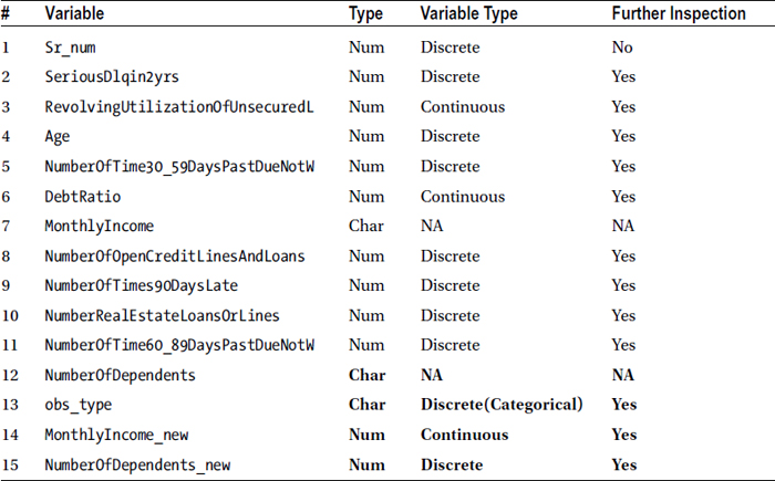
After going through the checklist of PROC CONTENTS, the following issues were found:
- There are two additional variables, Sr_num and obs_type.
- The monthly income and number of dependents should be numeric, but they are written as characters. This means that no arithmetic or numerical operations are possible on these two variables. This issue can be detrimental to the analysis and might yield disastrous results in the later phases of the project.
- SeriousDlqin2yrs should be Y/N but is read as a number. Y/N might have been converted to 0/1.
The rest of the data exploration steps will be explored. The discrepancies will be examined closely and resolved. If the answers to these issues are not found, check with the data team on whether they are because of manual or system errors.
Step 2: Data Exploration and Validation Using Data Snapshot
The PROC CONTENTS data gave an overview of observations and variables. The next step is to examine the values in each variable. As discussed earlier, printing the whole data set is not practical; only a snapshot of the data is to be printed. A snapshot is a small portion of the data. It may be random 100 observations, the first 30 observations, or the last 50. There is no rule on the snapshot size. Basically, it is nothing but the printing of data with some restrictions.
![]() Warning Be careful while printing the data; never try to print a large data set. The computer system and software may hang, and a reboot may be the only option to bring it back.
Warning Be careful while printing the data; never try to print a large data set. The computer system and software may hang, and a reboot may be the only option to bring it back.
The SAS code to print the first 20 records follows:
title'Proc Print on raw data (first 20 observations only)';
proc print data=WORK.cust_cred_raw (obs=20) ;
run;
Table 7-16 lists the output for this code.
Table 7-16. The First 20 Observations in the cust_cred_raw Data Set

Validation and Checkpoints in the Data Snapshot
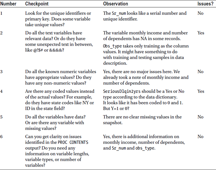
A snapshot is a cursory look at part of the actual data. This helps you understand the variables by looking at values they take. The following are the checkpoints that need to be observed in the PROC PRINT step:
- Look for the unique identifiers or primary key. Does some variable take unique values?
- Do all the text variables have relevant data? Or do they have some unexpected text in between, such as @!$# or &&&&.
- Do all the known numeric variables have appropriate values? Do they have non-numeric values also?
- Are there any coded values instead of the actual values? Examples are state codes like NY or ID in the state field.
- Do all the variables have data? Or is there any variable with missing values?
- Are the issues identified in the PROC CONTENTS output clear? This includes any information on variable lengths, variable types, number of variables, and so on.
Go through the checklist (Table 7-17) for the customer loan data.
Table 7-17. Checkpoints in the Customer Loan Data
The following are some open issue items from the contents:
- There are two additional variables: Sr_num and obs_type.
- The monthly income and number of dependents should be numeric but are written as characters.
- SeriousDlqin2yrs should be Y/N but is read as a number. Y/N might have been converted to 0/1.
From the snapshot, it was observed that Sr_num is a serial number, and the following code is a test to confirm this. A detailed analysis on Sr_num, using procunivariate, will reveal the facts.
Title 'Univariate on Sr_num';
proc univariate data=WORK.cust_cred_raw;
var sr_num;
run;
Table 7-18 provides a closer look at the quartiles and extreme values in the output.
Table 7-18. The Quartile and Extreme Observations in the cust_cred_raw Data Set
|
Quantiles (Definition 5) | |
|---|---|
|
Quantile |
Estimate |
|
100% Max |
251503 |
|
99% |
248988 |
|
95% |
238928 |
|
90% |
226353 |
|
75% Q3 |
188628 |
|
50% Median |
125752 |
|
25% Q1 |
62876 |
|
10% |
25151 |
|
5% |
12576 |
|
1% |
2516 |
|
0% Min |
1 |

The five highest values of sr_num are 251499, 251500, 251501, 251502, and 251503, and sr_num starts with 1, 2, 3, 4, and 5. Hence, it can be safely concluded that sr_num is the record number.
Resolving the Monthly Income and Number of Dependents Issue
Here are the burning open items:
- For obs_type, proc print didn’t give much information.
- The monthly income and number of dependents should be numeric, but they are written as characters.
- SeriousDlqin2yrs should be Y/N but is read as a number. Y/N might have been converted to 0/1.
Both monthly income and number of dependents are NA. As a result, the whole variable is stored as a character variable. Convert them to numerical missing values. Use if-then-else in SAS or the following code:
/* Monthly income & number of dependents Character issue*/
Data cust_cred_raw_v1;
Set cust_cred_raw;
MonthlyIncome_new= MonthlyIncome*1;
NumberOfDependents_new=NumberOfDependents*1;
run;
This creates two new variables, MonthlyIncome_new and NumberOfDependents_new, and creates a new data set called cust_cred_raw_v1 from old data set cust_cred_raw.
Some warning notes about NA multiplied by 1 are noticeable while executing the code. The log file will have messages similar to the following lines:
NOTE: Character values have been converted to numeric values at the places given by:
      (Line):(Column).
      71:21   72:24
NOTE: Invalid numeric data, MonthlyIncome='NA' , at line 71 column 21.
NOTE: Invalid numeric data, NumberOfDependents='NA' , at line 72 column 24.
Two new variables were created to resolve the character-related issues. The following is the PROC CONTENTS output of the new data set:
title'Proc Contents on data version1';
proc contents data=cust_cred_raw_v1 varnum ;
run;
Table 7-19 lists the output of this code.
Table 7-19. Output of proc contents on the cust_cred_raw_v1 Data Set

Two new numeric variables have been added, and they can now be used instead of character variables.
The following are the open items:
- For obs_type, PROC PRINT didn’t give sufficient information.
- SeriousDlqin2yrs should be Y/N but is read as a number. Y/N might have been converted to 0/1. What is 0 and what is 1 need to be decided.
PROC PRINT and the snapshot gave access to the real values, using certain issues that could be identified and resolved. The data issues may not be obvious in all the variables. For example, it is apparent that obs_type has something to do with test and training data, but PROC PRINT did not put forth a clear picture. Sometimes, increasing the print size will give a closer look at the values. Printing four or five parts of the data is usually sufficient to get a better picture.
The Continuous and Discrete Variables
The earlier chapters discussed continuous and discrete variables. A variable that can take any value between two limits is continuous (for example, height in feet). A variable that can take only limited values is called discrete (for example, number of children in a family). Time from an analog watch is a continuous variable, and time from a digital watch is a discrete variable. Both of them show time, but in an analog watch precision is not fixed, and a digital watch shows the time only to its lowest unit of measure, which can even be 100th of a second.
Table 7-20 shows the categorization of the variables into continuous and discrete in the given data.
Table 7-20. Discrete and Continuous Variables in the Data
After running the basic contents and printing procedures, comes descriptive statistics. As discussed earlier, there are no shortcuts. Every variable needs to be examined individually. Everything needs to be explored and validated before analysis. The first step in basic descriptive analysis is to identify the continuous and discrete variables. Since the continuous variables can take infinite values, components like a frequency table will be really long. On the other hand, discrete variables take a countable number of values, so a frequency table makes some sense.
The next step is to perform a univariate analysis on the continuous variables and frequency tables for discrete variables. A frequency table for continuous variables is not a good idea because it can take an infinite number of values, but it can be useful for discrete variables.
Step 3: Data Exploration and Validation Using Univariate Analysis
A univariate analysis is almost like a complete report on a variable and covers details from every angle. The univariate analysis will be used here to explore and validate all continuous variables. This analysis gives the output on the following statistical parameters:
- N (a count of non-missing observations)
- Nmiss (a count of missing observations)
- Min, max, median, mean
- Quartile numbers and percentiles (P1, p5, p10, q1(p25), q3(p75), p90, p99)
- Stdde (standard deviation)
- Var (variance)
- Skewness
- Kurtosis
Skewness and kurtosis deal with variable distribution. These two measures will not be used in this analysis. Here is a quick explanation of them for the sake of completeness.
Skewness explains on which side the most variable distribution is skewed. A negative skewness means the left side tail is longer when a distribution plot of the variable is drawn. Consider a variable, say the age of people with natural deaths; for most of such cases age will be really high. Similarly, a right-skewed distribution may feature a tail on the right side. The number of accidents in one’s life may be an example of right-skewed distribution. Look at Figures 7-2 and 7-3.

Figure 7-2. Left-skewed variable
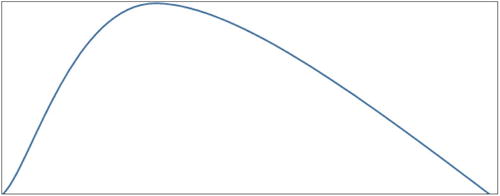
Figure 7-3. Right-skewed variable
Kurtosis details how well the variable is distributed in terms of the sharpness of the peak. The following figures show three different types of peaks. Figure 7-4 shows a sharp peak at one value. Figure 7-5 has almost no peak, and Figure 7-6 has a medium peak. The kurtosis measure value for the first graph will be in excess of 3; the kurtosis value will be much less than 3 for the second graph, and for the third variable, the kurtosis will be close to 3.

Figure 7-4. High kurtosis

Figure 7-5. Low kurtosis
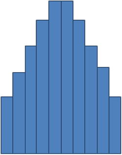
Figure 7-6. Medium kurtosis
The SAS code that follows is for conducting univariate analysis on variableRevolvingUtilizationOfUnsecuredL. More variables might be added if required, but you will start with one variable.
![]() Note To recap, RevolvingUtilizationOfUnsecuredL is a total balance on credit cards and personal lines of credit except real estate and the number of installment debt such as car loans divided by the sum of credit limits.
Note To recap, RevolvingUtilizationOfUnsecuredL is a total balance on credit cards and personal lines of credit except real estate and the number of installment debt such as car loans divided by the sum of credit limits.
Consider a credit card with $100,000 as a credit limit. If $25,000 is used on average every month, the utilization percentage is 25 percent. If $10,000 is used on average, the utilization is 10 percent. Hence, utilization takes values between 0 and 1 (that is, 0 to 100 percent).
Title 'Proc Univriate on utilization -RevolvingUtilizationOfUnsecuredL ';
Proc univariate data= cust_cred_raw_v1;
Var RevolvingUtilizationOfUnsecuredL;
run;
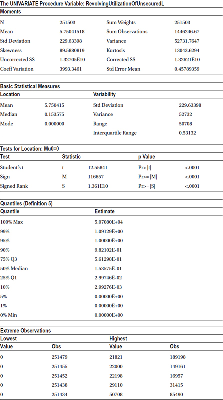
This code gives the output shown in Table 7-21.
Table 7-21. Output of proc univariate on cust_cred_raw_v1 (Var RevolvingUtilizationOfUnsecuredL)
Validation and Checkpoint in Univariate Analysis
The univariate analysis gives almost all measures of central tendency and . Here is the checklist for univariate analysis:
- What are the central tendencies of the variable? What are the mean, median, and mode across each variable? Is the mean close to the median?
- Is the concentration of variable as expected? What are quartiles? Is the variable skewed toward higher values? Or is it skewed toward lower values? What is the quartiles distribution? Are there any indications of the presence of outliers?
- What is the percentage of missing values associated with the variable?
- Are there any outliers/extreme values for the variable?
- What is the standard deviation of this variable? Is it near 0, or is it too high? Is the variable within the limits or possible range?
Table 7-22 contains the observations on the output.
Table 7-22. Observations on the Output of the Variable RevolvingUtilizationOfUnsecuredL

The output clearly indicates the presence of outliers, and these 5 percent outliers are inducing drastic errors in all the measures. One such example is the mean utilization of overall customers of 500 percent, whereas the actual average is 15 percent. The outliers can also be verified using a box plot. The “plot” option needs to be mentioned in the PROC UNIVARIATE code to create the box-plot graph:
title'ProcUnivriate and boxplot on utilization’;
Procc univariate data= cust_cred_raw_v1 plot;
Var RevolvingUtilizationOfUnsecuredL;
run;
Figure 7-7 shows the resulting box plot.

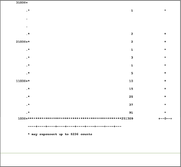
Figure 7-7. Box plot on the variable RevolvingUtilizationOfUnsecuredL
The box cannot be seen in the preceding box-plot graph; recall the box-plot interpretation: a box has Q1, median, and Q3. It is evident from the graph that the variable is completely dominated by outliers. To verify further, consider values only below 100 percent. The SAS code and output will look like the following:
title'Proc Univariate on utilization less than or equal to 100%';

Proc univariate data= cust_cred_raw_v1 plot;
Var RevolvingUtilizationOfUnsecuredL;
Where RevolvingUtilizationOfUnsecuredL<=1;
run;
Table 7-23 and Figure 7-8 show PROC UNIVARIATE and the box plot on utilization less than or equal to 100 percent.
Table 7-23. Output of PROC UNIVARIATE on RevolvingUtilizationOfUnsecuredL<=1


Figure 7-8. The box plot of PROC UNIVARIATE on RevolvingUtilizationOfUnsecuredL<=1
You can see the box now. Although there are some high-side values, there are no relentless outliers in this case. But simply removing the outliers is not a solution. This needs to be noted and resolved later. There are two open items already, and the revolving utilization variable here contains outliers, which need to be treated. That is the third issue on the list.
- For obs_type, PROC PRINT didn’t give sufficient information.
- SeriousDlqin2yrs should be Y/N, but it is read as a number. It might be possible that Y/N is converted to 0/1. What is 0 and what is 1 need to be decided.
- Revolving utilization has outliers, around 5 percent.
Similarly, univariate analysis is performed on monthly income using this code:
title' Univariate on monthly income ';
Proc univariate data= cust_cred_raw_v1 ;
Var MonthlyIncome_new;
run;
Table 7-24 shows the output of this code.
Table 7-24. Output of proc univariate on cust_cred_raw_v1 (Var MonthlyIncome_new)
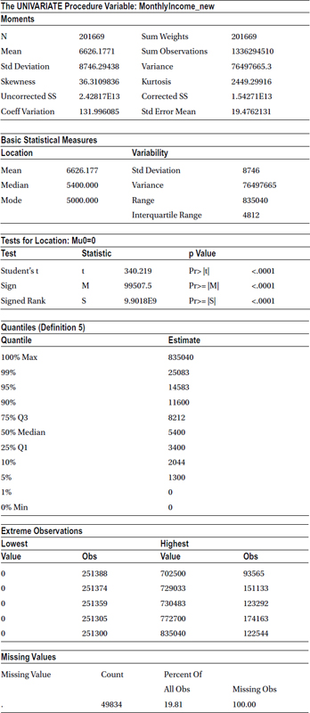
There are outliers in monthly income because the mean is slightly higher than the median, and these outliers are on the higher side of values taken by this variable. But a serious issue other than the mild outliers is that the variable has some missing values, almost 49,834. That is, 20 percent of the overall monthly income records are missing. This is detrimental to the analysis. SAS will ignore this 20 percent of the records whenever monthly income is used. This is the fourth issue on the following list:
- For obs_type, Proc print didn’t give sufficient information.
- SeriousDlqin2yrs should be Y/N, but it is read as a number. It might be possible that Y/N is converted to 0/1. What is 0 and what is 1 need to be decided.
- Revolving utilization has outliers, around 5 percent.
- The monthly income is missing in nearly 20 percent of the cases.
Similarly, univariate analysis can be performed on all the continuous variables; they can be validated, and the issues can be recorded.
Step 4: Data Exploration and Validation Using Frequencies
Step 4 inspects all the discrete variables that take a countable number of values. A frequency table should be created only for discrete and categorical variables. A frequency table on a continuous variable can hang your system, since you expect continuous variables to take an almost infinite number of values. So, if you have too many records in the data, you need to be careful while choosing the variables for frequency distributions.
The following is the code for frequency tables for SeriousDlqin2yrs and obs_type. Once we show the frequency tables, we will explain how they can be used to your advantage.
Title 'Frequency table for  Serious delinquency in 2 years ';
proc freq data= cust_cred_raw_v1;
table SeriousDlqin2yrs;
run;
Table 7-25 gives the output for this code.
Table 7-25. Output of proc freq on the cust_cred_raw_v1 Data Set (Table SeriousDlqin2yrs)

|
Frequency Missing = 101503 |
The output is missing in 101,503 values. The count of missing values is given in the output of PROC FREQ. It has already been mentioned by the data team that the serious delinquency values are not available for the testing population. If a proc frequency is run on obs_type, it should yield exactly 101,503 testing records.
title' Frquency table for  obs_type ';
proc freq data=    cust_cred_raw_v1;
table obs_type;
run;
Table 7-26 lists the output for this code.
Table 7-26. Output of proc freq on the cust_cred_raw_v1 Data Set (Table obs_type)
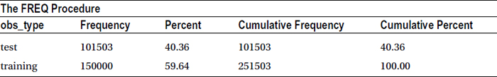
Hence, 150,000 observations will be used for model building, and the rest will be used for testing. Obs_type simply indicates the testing and training records.
A frequency table of the other discrete variable will also be created. The serious delinquency variable is 0 for 93.3 percent of the records and is 1 for 6.7 percent of the records. The second issue on the list can be resolved by applying some banking knowledge. Serious delinquencies are generally fewer than nondelinquencies. A good customer base of 93 percent and the bad customer base of 7 percent can be expected in a borrower population, but the other way around is almost impossible. So, it can safely be inferred that Y is coded as 1 and N is coded as 0.
That leaves two remaining issues on the list:
- Revolving utilization has outliers of around 5 percent.
- The monthly income is missing in 20 percent of the cases.
The following is a continuation of the frequency table for NumberOfTime30_59DaysPastDueNotW. The variable indicates how many times a customer is delinquent for one month but no later than 59 days. A customer can default possibly once, twice, and a maximum of 24 times in a 24-month period. A maximum of 24 times in a 24-month period would mean that the customer has defaulted in a bill payment every month.
The following is the code for the frequency table of this variable:
title' Frquency table for  30-59 days past due ';
proc freq data=    cust_cred_raw_v1;
table NumberOfTime30_59DaysPastDueNotW;
run;
Table 7-27 lists the output of this code.
Table 7-27. Output of proc freq on cust_cred_raw_v1 (Table NumberOfTime30_59DaysPastDueNotW)

Validation and Checkpoints in Frequencies
The following are the points that can be considered using variable frequency tables for data validation and exploration:
- Are the values as expected?
- Is the variable concentration as expected?
- Are there any missing values? What is the percentage of missing values?
- Are there any extreme values or outliers?
- Is there a possibility of creating a new variable that has a small number of distinct categories by grouping certain categories with others?
Table 7-28 shows the observations of the output of 30 to 59 DPD (days past due).
![]() Note To recap, 30 to 59 DPD is the short form used for the variable defined earlier: NumberOfTime30-59DaysPastDueNotWorse. It is the number of times the borrower has been 30 to 59 DPD days past due, but no worse, in the last 2 years.
Note To recap, 30 to 59 DPD is the short form used for the variable defined earlier: NumberOfTime30-59DaysPastDueNotWorse. It is the number of times the borrower has been 30 to 59 DPD days past due, but no worse, in the last 2 years.
Table 7-28. Observations of the Output of 30 to 59 DPD

There are two more variables similar to 30 to 59 DPD: 60 to 89 DPD and 90 DPD.
![]() Note To recap, 60 to 89 DPD is the variable NumberOfTime60-89DaysPastDueNotWorse. It is the number of times the borrower has been 60 to 89 days past due, but no worse, in the last 2 years.
Note To recap, 60 to 89 DPD is the variable NumberOfTime60-89DaysPastDueNotWorse. It is the number of times the borrower has been 60 to 89 days past due, but no worse, in the last 2 years.
90 DPD is the variable NumberOfTimes90Days. It is the number of times the borrower has been 90 days or more past due. This data is for 2 years. How many times was a customer 90 days late but not worse? One, two, three, or five times?
Consider the following code, which gives frequency tables for 60 to 89 DPD and 90 DPD:
title' Frquency table for  60-89, and 90+ days past due ';
proc freq data=    cust_cred_raw_v1;
table NumberOfTime60_89DaysPastDueNotW     NumberOfTimes90DaysLate;
run;
Table 7-29 shows the output of this code.
Table 7-29. Frequency Tables for 60 to 89 and 90+ Days Past Due


The issue of 96 and 98 seems to be consistent. Are these default values? The percentage will pose a problem despite it being a low value. This has to be taken note of before resolving.
The list of issues now includes the following:
- Revolving utilization has outliers of around 5 percent.
- The monthly income is missing in 20 percent of the cases.
- 30 to 59 DPD, 60 to 89 DPD, and 90 DPD have issues with 96 and 98.
Similarly, frequency tables have to be created for all the variables in order to fully understand the complete data set. The following code gives the frequency tables for other variables as well:
Proc freq data=cust_cred_raw_v1;
tables
age
NumberOfOpenCreditLinesAndLoans
NumberRealEstateLoansOrLines
NumberOfDependents_new;
run;
Table 7-30 is the frequency table for NumberOfDependents_new. You will have similar frequency tables for the remaining variables, which are not shown here.
Table 7-30. Frequency Table for NumberOfDependents_new

|
Frequency Missing = 6550 |
The variable values in the preceding output are missing 2 percent of the observations. This is an issue. As given in the following code, the missing option can be used to see the missing percentage in proc frequency:
title' Frequency  table for All discrete variables with missing %';
proc freq data=cust_cred_raw_v1  ;
tables
age NumberOfOpenCreditLinesAndLoans NumberRealEstateLoansOrLines
NumberOfDependents_new/missing;
run;
Table 7-31 is the frequency table for NumberOfDependents_new with this code. You will have similar frequency tables for the remaining variables, which are not shown here.
Table 7-31. Frequency Table for NumberOfDependents_new with /missing Option

The list of issues so far is as follows:
- Revolving utilization has outliers of around 5 percent.
- The monthly income is missing in 20 percent of the cases.
- 30 to 59 DPD, 60 to 89 DPD, and 90 DPD have an issue with 96 and 98.
- The number of dependents is missing around 2 percent of values.
The completion of contents, print, univariate analysis, and frequency steps may be the end of data exploration and validation. Conducting all these steps on some variables brought forth the preceding four issues. Similar issues can be found with other variables as well. Make notes of them and move on to the next step of cleaning the data. This is also called preparing the data for analysis. Having outliers is certainly an issue, but removing them is not the solution.
After data exploration and data validation, these questions are left unanswered:
- Some variables have missing values/outliers, but those records cannot be dropped.
- Some variables have a high percentage of missing values/outliers. Can they be dropped?
- Some variables have negligible missing values/outliers. How should they be treated when there are 2 percent, 40 percent, and 95 percent missing values?
- Can the missing values be substituted with some other values?
- Some variables are discrete and some continuous. Is the treatment (dropping or substitution) the same for discrete and continuous variables? If a continuous variable has 20 percent missing values and a discrete variable, which has just four levels, also has 20 percent missing values, can they be treated the same?
With these questions in mind, you can now proceed to the next step in the data preparation process.
Step 5: The Missing Value and Outlier Treatment
It has already been established that dropping the records because of missing values is not a good solution. Instead, a technique called imputation might be used. This technique involves replacing missing/erroneous values with the best possible substitutions to minimize the damage yet get accurate results. There are different types of imputations; we’ll discuss two: stand-alone and those based on related variables.
The missing values need to be replaced with either the mean or median, depending on the rest of the values and what makes better business sense. The stand-alone imputation is convenient and easy to implement. The assumption here is that the missing values are not very distinct from the values that are already present.
The data in Table 7-32 shows the age of 21 athletes; one athlete’s age is missing. Replace the missing value with 27, which is the average age of the rest of the values, since only one value is missing. (In general, the age of an athlete will be no more than 50 or 60.)
Table 7-32. Age Data for Athletes
![]()
The new data will look like Table 7-33 after stand-alone imputation (using mean of the rest of the age values to replace the missing value).
Table 7-33. Age Data for Athletes After Stand-Alone Imputation
![]()
The stand-alone imputation is a good method to use if small portions of the data are missing or fall into the category of outliers.
Imputation Based on Related Variable
In some cases, the relation between the variables might be used to impute. Consider the data given in Table 7-34, where the number of games and ages of athletes are shown as two columns.
Table 7-34. Age vs. Appearances for Athletes
|
Age |
Appearances |
|---|---|
|
25 |
201 |
|
32 |
265 |
|
25 |
206 |
|
19 |
154 |
|
23 |
193 |
|
31 |
257 |
|
178 | |
|
37 |
301 |
|
33 |
268 |
|
28 |
229 |
|
24 |
194 |
|
31 |
251 |
|
30 |
247 |
|
36 |
295 |
|
38 |
312 |
|
26 |
213 |
|
40 |
330 |
|
26 |
209 |
|
40 |
330 |
|
20 |
162 |
|
35 |
283 |
|
22 |
177 |
The age is missing for one athlete. If stand-alone imputation is used, an average age of 30 is derived. To determine whether the missing value can be replaced with 30, the information on the number of games played can be used. A simple sort on the number of games produces Table 7-35.
Table 7-35. Age vs. Appeareances for Athletes After Sorting
|
Age |
Appearances |
|---|---|
|
40 |
330 |
|
40 |
330 |
|
38 |
312 |
|
37 |
301 |
|
36 |
295 |
|
35 |
283 |
|
33 |
268 |
|
32 |
265 |
|
31 |
257 |
|
31 |
251 |
|
30 |
247 |
|
28 |
229 |
|
26 |
213 |
|
26 |
209 |
|
25 |
206 |
|
25 |
201 |
|
24 |
194 |
|
23 |
193 |
|
178 | |
|
22 |
177 |
|
20 |
162 |
|
19 |
154 |
The number of games infers that 22 is a better value than 30. Imputation based on variable relation is definitely a better method, but what are the variables to be considered while making the imputations? To answer this question, you need to have a clear idea of all variables and business problems at hand. As discussed in the following section, in all the cases of missing values, imputation may not be the best technique.
Imputation will not work as well if there are too many missing values (Table 7-36). For example, if 70 percent of the values in a variable are missing, they cannot be imputed based on the remaining 30 percent of values. In this case, creating an indicator variable (Table 7-37) to tell whether the parent value is missing or present is the only workable solution.
Table 7-36. Example of Too Many Missing Values in Data
![]()
Table 7-37 shows the best that can be taken out of the variable that is listed in Table 7-36.
Table 7-37. Indicator Variable for Table 7-36
![]()
Hence, when there are too many missing values, the actual variable should be dropped and replaced with an indicator variable.
The Missing Value and Outlier Treatment
Earlier topics explained how to explore and validate the variables. A few issues with missing values and outliers were found while validating the data. The chart in Figure 7-9 shows the missing value and outlier treatment for both continuous and discrete variables for all levels of missing value percentages. You can first start with missing value treatment and then move on to outlier treatment. The same order applies, if a variable has both missing values and outliers.

Figure 7-9. How to treat missing value and outliers
This chart can be used for cleaning the data. There are two types of variables: discrete and continuous. The percentage missing in each variable might be different.
Practically speaking, the following are the possible percentages of missing values in discrete and continuous variables:
- A discrete variable with less than 10 percent of missing values or outliers
- A discrete variable with 10 to 50 percent of missing values or outliers
- A discrete variable with more than 50 percent of missing values or outliers
- A continuous variable with less than 10 percent of missing values or outliers
- A continuous variable with 10 to 50 percent of missing values or outliers
- A continuous variable with more than 50 percent of missing values or outliers
The treatment for each situation follows.
For a discrete variable with less than 10 percent of missing values or outliers:
- It is best to impute based on a related variable. Since a discrete variable has levels, stand-alone imputation may not be effective.
- Consider the example Table 7-38 for the variable number of savings accounts held by customers.
Table 7-38. Number of Savings Accounts Held by Customers
|
Number of Accounts |
Number of Customers |
|---|---|
|
0 |
2,505 |
|
1 |
351,234 |
|
2 |
339,778 |
|
3 |
139,918 |
|
4 |
124,044 |
|
5 |
94,003 |
|
6 |
74,325 |
|
7 |
64,469 |
|
8 |
1,456 |
|
#N/A |
34,530 |
|
Total |
1,226,262 |
Of the total number of customers, 34,530 customers’ data is missing. The number of accounts they hold is not specified. It is almost 2.8 percent of the total data. A stand-alone imputation performed on the data yields 2.7 as the average number of accounts in the population. It can simply be inferred that 34,530 customers have three accounts each, or some other related variable can be made use of.
Sound business insight is necessary to pick the best related variable to perform an imputation. This example considers one more variable called the credit card holder indicator. It takes just two values, Yes or No. Say you are trying to use this indicator to perform the imputation. How this can be done? For this, you need some more information.
Out of 1,226,262 customers, some have credit cards, and some of them don’t have any. Table 7-39 still shows frequency of customers with 1,2,3,4, and 8 savings accounts. Out of 351,234 customers with one savings account, how many of them have credit cards? How many don’t have any card? There are 339,778 customers with two savings accounts, so how many of them have a credit card? How many of them don’t have any card? These questions will be answered using a simple cross-tab association table between the number of accounts and credit card indicator.
Table 7-39. Frequency of Customers with Savings Accounts and Credit Cards (Data Filled in Table 7-40)

The cross-tab association table shown in Table 7-40 between the numbers of saving accounts will determine what the right substitution for N/A might be.
Table 7-40. Frequency of Customers with Savings Accounts and Credit Cards

Table 7-41 shows the same table in terms of percentages.
Table 7-41. Freqeuncy of Customers with Savings Accounts and Credit Cards (% Values)

Of the total number of customers who have one savings account each, 70 percent have at least one credit card. Similarly, 81 percent of customers with four savings accounts each have credit cards. In the group with the number of savings account as N/A, only 1 percent has credit cards, and the rest of the 99 percent don’t have any credit card. The same is the case with the number of savings accounts = 0 group.
One percent of customers with 0 and N/A savings accounts are credit card holders. Hence, a good solution is replacing N/A with 0, rather than an overall mean of 3. This is imputation with respect to another related variable. There is no rule of thumb to select a related variable; it depends on the business problem that is being solved.
For a discrete variable with 10 to 50 percent missing values or outliers:
- Two tasks need to be performed in this case: imputing the missing values based on related variable and creating a dummy/indicator variable with a missing (as 1) vs. nonmissing category.
- The first task is ensuring that there are no missing values. Make sure that missing/nonmissing records are flagged in the data since a considerable portion of the data is missing. A new indicator variable that will capture the information regarding missing and nonmissing records of a variable needs to be created. This will be used in analysis later. How to create an indicator variable was already explained in the earlier sections. The second task is to impute the missing value based on a related variable.
For a discrete variable with more than 50 percent missing values or outliers:
A new indicator variable needs to be created and the original variable dropped because the minuscule percentage of the available values cannot be used.
For a continuous variable with less than 10 percent missing values or outliers:
A stand-alone imputation, is sufficient.
For a continuous variable with 10 to 50 percent missing values or outliers:
Both indicator variables need to be created and missing values should be imputed.
For a continuous variable with more than 50 percent missing values or outliers:
Create an indicator variable and drop the original variable.
Turning back to the case, the issues so far are as follows:
- Revolving utilization, which is a continuous variable, has outliers around 5 percent.
- The monthly income is a continuous variable and has missing values in 20 percent of the cases.
- 30 to 59 DPD, 60 to 89 DPD, and 90 DPD are all discrete variables; values 96 and 98 have issues. The percentage of such errors is less than 10 percent.
- The number of dependents is a discrete variable and has around 2 percent missing values.
The following sections examine what type of issue a variable has and perform the right treatment on the variable.
Cleaning Continuous Variables
In previous sections, you found outliers in variable RevolvingUtilizationOfUnsecuredL. Now you will try to treat them.
Let’s start with the variable Revolving Utilization (RevolvingUtilizationOfUnsecuredL). Given in Table 7-42 is the proc univariate output for this variable, as taken from Table 7-21.
Table 7-42. Quantiles Table from the Univariate Output of RevolvingUtilizationOfUnsecuredL
|
Quantiles (Definition 5) | |
|---|---|
|
Quantile |
Estimate |
|
100% Max |
5070800% |
|
99% |
109% |
|
95% |
100% |
|
90% |
98% |
|
75% Q3 |
56% |
|
50% Median |
15% |
|
25% Q1 |
3% |
|
10% |
0% |
|
5% |
0% |
|
1% |
0% |
|
0% Min |
0% |
Revolving Utilization, which is a continuous variable, has outliers of around 5 percent. Refer to Figure 7-10.
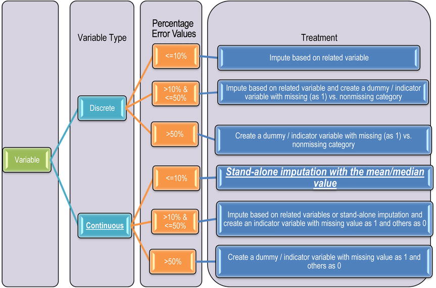
Figure 7-10. Treating continuous variables for 5 percent outliers
The mean value of utilization after ignoring outliers can be found by using the following code:
Title 'Proc Univariate on utilization less than or equal to 100% ';
Proc univariate data= cust_cred_raw_v1 plot;
Var RevolvingUtilizationOfUnsecuredL;
Where RevolvingUtilizationOfUnsecuredL<=1;
run;
Table 7-43 lists the output of this code.
Table 7-43. Output of proc univariate with RevolvingUtilizationOfUnsecuredL<=1

Since the outliers have been removed, the new mean of 30.4 percent is the actual central tendency and can be used. Stand-alone imputation is performed in the following code by replacing the outliers with mean values:
title'Treating utilization ';
data  cust_cred_raw_v2;
set cust_cred_raw_v1;
if RevolvingUtilizationOfUnsecuredL>1then utilization_new=0.304325;
else utilization_new= RevolvingUtilizationOfUnsecuredL;
run;
The preceding code creates a new data set called cust_cred_raw_v2 using cust_cred_raw_v1; a new variable called utilization_new is created in such a way that if RevolvingUtilizationOfUnsecuredL is greater than 1 (that is, 100 percent), then utilization_new is the mean of RevolvingUtilizationOfUnsecuredLie, which is 0.304325. Otherwise, it is the same as the old value.
The log file for preceding code looks like this:
NOTE: There were 251503 observations read from the data set WORK.CUST_CRED_RAW_V1.
NOTE: The data set WORK.CUST_CRED_RAW_V2 has 251503 observations and 16 variables.
NOTE: DATA statement used (Total process time):
real time           0.84 seconds
cpu time            0.40 seconds
The following is the new variable’s univariate analysis:
Title 'New utilization univariate ';
Proc univariate data= cust_cred_raw_v2 plot;
Var utilization_new;
run;
The output of this code is given in Table 7-44 and Figure 7-11.
Table 7-44. Output of proc univariate on utilization_new Variable

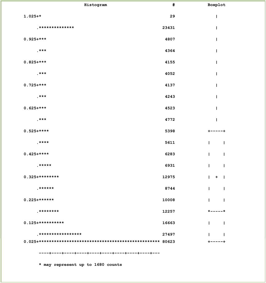
Figure 7-11. Box plot for utilization_new variable
utilization_new will be used for analysis henceforth. The issue with the outliers is now resolved. In the next section, you will treat monthly income, which has 20 percent missing values.
Treating Monthly Income
The monthly income is a continuous variable and is missing values in 20 percent of the data. Refer to Figure 7-12.

Figure 7-12. Treating a continuous variable with 20 percent missing values
Since the monthly income is continuous and is missing 20 percent of the values, a monthly income indicator variable needs to be created, and the missing values with the median will be imputed, as shown in the following code:
title'Treating Monthly income ';
data  cust_cred_raw_v2;
set  cust_cred_raw_v2;
if    MonthlyIncome_new =.then    MonthlyIncome_ind =1 ;
else MonthlyIncome_ind = 0;
run;
The preceding code creates a new variable called MonthlyIncome_ind, which takes value 1, when MonthlyIncome_new is . (a missing value), otherwise 0.
The following code creates a new variable called MonthlyIncome_final, which takes a value of 5400 when MonthlyIncome_new is . (a missing value). Otherwise, the new variable is the same as the old variable. This only replaces missing values with the mean.
data  cust_cred_raw_v2;
set  cust_cred_raw_v2;
if    MonthlyIncome_new =.then    MonthlyIncome_final=5400.000 ;
else MonthlyIncome_final = MonthlyIncome_new;
run;
Now, in the following code, you are performing univariate analysis on the monthly income variable after the treatment. Everything seems to falls into place now.
title'Univariate Analysis on Final  Monthly income ';
Proc univariatedata= cust_cred_raw_v2 ;
Var MonthlyIncome_final;
run;
Table 7-45 shows the output of this code.
Table 7-45. Monthly Income After Resolving the Missing Values Issues (proc univariate on MonthlyIncome_final)
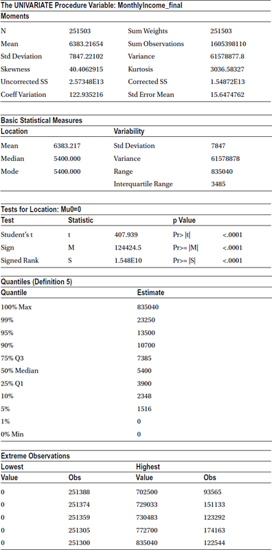
The monthly income variable is cleaned now. We can use these two new variables for the analysis from here on.
30 to 59 DPD, 60 to 89 DPD, and 90 DPD are all discrete variables. They have issues with the values 96 and 98. The percentage of such errors is less than 10 percent. Figure 7-13 gives the solution.

Figure 7-13. Treating a discrete variable with less than 10 percent error values
The treatment for this variable is imputation based on a related variable. Experience/observation shows the distribution of 30 DPD in combination with serious delinquency, which is the target variable and the most important of all. The cross-tab frequency of serious delinquency (the bad indicator), and 30 DPD is found in the following code:
Title 'Cross tab frequency of NumberOfTime30_59DaysPastDue1 and SeriousDlqin2yrs';
proc freq data=cust_cred_raw_v2;
tables NumberOfTime30_59DaysPastDueNotW*SeriousDlqin2yrs;
run;
Table 7-46 gives the output of the preceding code.
Table 7-46. The Cross-Tab Frequency of NumberOfTime30_59DaysPastDueNotW*SeriousDlqin2yrs


The cross-tab frequency shows overall frequency, overall percent, row percent, and column percent of that value. The percentage of zeros in class 98 is 45.83, and the nearest group with a percent of zeros is group 6, in other words, 47.14. So, the bad rate in group 98 is 54 percent, and the nearest group with a bad rate is 52.8 percent. The apt substitution for 98 will be 6, since there is no other group whose bad rate is similar to this group. Since group 6 is admissible and has a bad rate of 52.8 percent, 98 can be safely replaced with 6. Since there are just five observations in 96, both 96 and 98 can be replaced with 6.
The following code simply creates a new variable that takes value 6 when 30 DPD is 96 or 98. Otherwise, it is the same as 30 DPD.
title'Treating 30DPD';
data cust_cred_raw_v2;
set   cust_cred_raw_v2;
if    NumberOfTime30_59DaysPastDueNotW in (96, 98) then    NumberOfTime30_59DaysPastDue1= 6;
else  NumberOfTime30_59DaysPastDue1= NumberOfTime30_59DaysPastDueNotW;
run;
In the preceding code, a new variable called NumberOfTime30_59DaysPastDue1 is created based on NumberOfTime30_59DaysPastDueNot. The new variable takes a value of 6 whenever NumberOfTime30_59DaysPastDueNotW takes 96 or 98. Otherwise, it is same as the old variable.
The following is the log file and output:
NOTE: There were 251503 observations read from the data set WORK.CUST_CRED_RAW_V2.
NOTE: The data set WORK.CUST_CRED_RAW_V2 has 251503 observations and 19 variables.
NOTE: DATA statement used (Total process time):
real time           0.60 seconds
cpu time            0.49 seconds
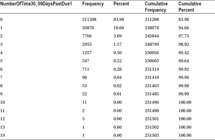
The new variable is now free from errors. The following code runs PROC FREQUENCY on the variable NumberOfTime30_59DaysPastDue1:
Proc freq data=cust_cred_raw_v2;
tables NumberOfTime30_59DaysPastDue1;
run;
Table 7-47 gives the output of this code.
Table 7-47. Output of proc freq on NumberOfTime30_59DaysPastDue1
Similarly, the rest of the variables can be treated using the treatment chart depicted in Figure 7-13. Once we are done with all the variables and finish all the exploration, validation, and cleaning steps, the data is ready for analysis.
![]() Note The previous treatment chart, represented in Figure 7-13, is suggestive only; a slightly different approach for outliers can also be used. When the outliers are 10 to 50 percent, they can be treated as a different class, or a subset can be taken for the population. This depends on the problem objectives at hand.
Note The previous treatment chart, represented in Figure 7-13, is suggestive only; a slightly different approach for outliers can also be used. When the outliers are 10 to 50 percent, they can be treated as a different class, or a subset can be taken for the population. This depends on the problem objectives at hand.
Conclusion
This chapter covered various ways of exploring and validating data. It also dealt with identifying issues in the data and then resolving them by using imputation techniques. As you can see, data cleaning requires a lot of time. Using junk data in analysis will only lead to useless insights. The methods provided here are guidelines rather than rules, and they arise from our work experience in the field. Using wisdom and rationale is important in preparing the data for analysis. Hence, the same amount of importance needs to be given to data cleaning as to data analysis. Preparing the data for analysis is the second step in analysis. Subsequent chapters will examine analysis and predictive modeling techniques.