![]()
Foundations of T-SQL
SQL Server 2014 is the latest release of Microsoft’s enterprise-class database management system (DBMS). As the name implies, a DBMS is a tool designed to manage, secure, and provide access to data stored in structured collections in databases. Transact-SQL (T-SQL) is the language that SQL Server speaks. T-SQL provides query and data-manipulation functionality, data definition and management capabilities, and security administration tools to SQL Server developers and administrators. To communicate effectively with SQL Server, you must have a solid understanding of the language. In this chapter, you begin exploring T-SQL on SQL Server 2014.
A Short History of T-SQL
The history of Structured Query Language (SQL), and its direct descendant Transact-SQL (T-SQL), begins with a man. Specifically, it all began in 1970 when Dr. E. F. Codd published his influential paper “A Relational Model of Data for Large Shared Data Banks” in the Communications of the Association for Computing Machinery (ACM). In his seminal paper, Dr. Codd introduced the definitive standard for relational databases. IBM went on to create the first relational database management system, known as System R. It subsequently introduced the Structured English Query Language (SEQUEL, as it was known at the time) to interact with this early database to store, modify, and retrieve data. The name of this early query language was later changed from SEQUEL to the now-common SQL due to a trademark issue.
Fast-forward to 1986, when the American National Standards Institute (ANSI) officially approved the first SQL standard, commonly known as the ANSI SQL-86 standard. The original versions of Microsoft SQL Server shared a common code base with the Sybase SQL Server product. This changed with the release of SQL Server 7.0, when Microsoft partially rewrote the code base. Microsoft has since introduced several iterations of SQL Server, including SQL Server 2000, SQL Server 2005, SQL Server 2008, SQL 2008 R2, SQL 2012, and now SQL Server 2014. This book focuses on SQL Server 2014, which further extends the capabilities of T-SQL beyond what was possible in previous releases.
Imperative vs. Declarative Languages
SQL is different from many common programming languages such as C# and Visual Basic because it’s a declarative language. In contrast, languages such as C++, Visual Basic, C#, and even assembler language are imperative languages. The imperative language model requires the user to determine what the end result should be and tell the computer step by step how to achieve that result. It’s analogous to asking a cab driver to drive you to the airport and then giving the driver turn-by-turn directions to get there. Declarative languages, on the other hand, allow you to frame your instructions to the computer in terms of the end result. In this model, you allow the computer to determine the best route to achieve your objective, analogous to telling the cab driver to take you to the airport and trusting them to know the best route. The declarative model makes a lot of sense when you consider that SQL Server is privy to a lot of “inside information.” Just like the cab driver who knows the shortcuts, traffic conditions, and other factors that affect your trip, SQL Server inherently knows several methods to optimize your queries and data-manipulation operations.
Consider Listing 1-1, which is a simple C# code snippet that reads in a flat file of names and displays them on the screen.
Listing 1-1. C# Snippet to Read a Flat File
StreamReader sr = new StreamReader("c:\Person_Person.txt");
string FirstName = null;
while ((FirstName = sr.ReadLine()) != null) {
Console.WriteLine(s); } sr.Dispose();
The example performs the following functions in an orderly fashion:
- The code explicitly opens the storage for input (in this example, a flat file is used as a “database”).
- It reads in each record (one record per line), explicitly checking for the end of the file.
- As it reads the data, the code returns each record for display using Console.Writeline().
- Finally, it closes and disposes of the connection to the data file.
Consider what happens when you want to add a name to or delete a name from the flat-file “database.” In those cases, you must extend the previous example and add custom routines to explicitly reorganize all the data in the file so that it maintains proper ordering. If you want the names to be listed and retrieved in alphabetical (or any other) order, you must write your own sort routines as well. Any type of additional processing on the data requires that you implement separate procedural routines.
The SQL equivalent of the C# code in Listing 1-1 might look something like Listing 1-2.
Listing 1-2. SQL Query to Retrieve Names from a Table
SELECT FirstName FROM Person.Person;
![]() Tip Unless otherwise specified, you can run all the T-SQL samples in this book in the AdventureWorks 2014 or SQL 2014 In-Memory sample database using SQL Server Management Studio or SQLCMD.
Tip Unless otherwise specified, you can run all the T-SQL samples in this book in the AdventureWorks 2014 or SQL 2014 In-Memory sample database using SQL Server Management Studio or SQLCMD.
To sort your data, you can simply add an ORDER BY clause to the SELECT query in Listing 1-2. With properly designed and indexed tables, SQL Server can automatically reorganize and index your data for efficient retrieval after you insert, update, or delete rows.
T-SQL includes extensions that allow you to use procedural syntax. In fact, you could rewrite the previous example as a cursor to closely mimic the C# sample code. These extensions should be used with care, however, because trying to force the imperative model on T-SQL effectively overrides SQL Server’s built-in optimizations. More often than not, this hurts performance and makes simple projects a lot more complex than they need to be.
One of the great assets of SQL Server is that you can invoke its power, in its native language, from nearly any other programming language. For example, in .NET you can connect to SQL Server and issue SQL queries and T-SQL statements to it via the System.Data.SqlClient namespace, which is discussed further in Chapter 16. This gives you the opportunity to combine SQL’s declarative syntax with the strict control of an imperative language.
SQL Basics
Before you learn about developments in T-SQL, or on any SQL-based platform for that matter, let’s make sure we’re speaking the same language. Fortunately, SQL can be described accurately using well-defined and time-tested concepts and terminology. Let’s begin the discussion of the components of SQL by looking at statements.
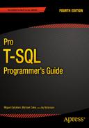
To begin with, in SQL you use statements to communicate your requirements to the DBMS. A statement is composed of several parts, as shown in Figure 1-1.
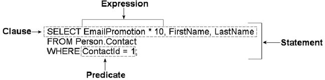
Figure 1-1. Components of a SQL statement
As you can see in the figure, SQL statements are composed of one or more clauses, some of which may be optional depending on the statement. In the SELECT statement shown, there are three clauses: the SELECT clause, which defines the columns to be returned by the query; the FROM clause, which indicates the source table for the query; and the WHERE clause, which is used to limit the results. Each clause represents a primitive operation in the relational algebra. For instance, in the example, the SELECT clause represents a relational projection operation, the FROM clause indicates the relation, and the WHERE clause performs a restriction operation.
![]() Note The relational model of databases is the model formulated by Dr. E. F. Codd. In the relational model, what are known in SQL as tables are referred to as relations; hence the name. Relational calculus and relational algebra define the basis of query languages for the relational model in mathematical terms.
Note The relational model of databases is the model formulated by Dr. E. F. Codd. In the relational model, what are known in SQL as tables are referred to as relations; hence the name. Relational calculus and relational algebra define the basis of query languages for the relational model in mathematical terms.
ORDER OF EXECUTION
Understanding the logical order in which SQL clauses are applied within a statement or query is important when setting your expectations about results. Although vendors are free to physically perform whatever operations, in any order, that they choose to fulfill a query request, the results must be the same as if the operations were applied in a standards-defined order.
The WHERE clause in the example contains a predicate, which is a logical expression that evaluates to one of SQL’s three possible logical results: true, false, or unknown. In this case, the WHERE clause and the predicate limit the results to only rows in which ContactId equals 1.
The SELECT clause includes an expression that is calculated during statement execution. In the example, the expression EmailPromotion * 10 is used. This expression is calculated for every row of the result set.
SQL THREE-VALUED LOGIC
SQL institutes a logic system that may seem foreign to developers coming from other languages like C++ or Visual Basic (or most other programming languages, for that matter). Most modern computer languages use simple two-valued logic: a Boolean result is either true or false. SQL supports the concept of NULL, which is a placeholder for a missing or unknown value. This results in a more complex three-valued logic (3VL).
Let’s look at a quick example to demonstrate. If I asked you, “Is x less than 10?” your first response might be along the lines of, “How much is x ?” If I refused to tell you what value x stood for, you would have no idea whether x was less than, equal to, or greater than 10; so the answer to the question is neither true nor false—it’s the third truth value, unknown. Now replace x with NULL, and you have the essence of SQL 3VL. NULL in SQL is just like a variable in an equation when you don’t know the variable’s value.
No matter what type of comparison you perform with a missing value, or which other values you compare the missing value to, the result is always unknown. The discussion of SQL 3VL continues in Chapter 3.
The core of SQL is defined by statements that perform five major functions: querying data stored in tables, manipulating data stored in tables, managing the structure of tables, controlling access to tables, and managing transactions. These subsets of SQL are defined following:
- Querying: The SELECT query statement is complex. It has more optional clauses and vendor-specific tweaks than any other statement. SELECT is concerned simply with retrieving data stored in the database.
- Data Manipulation Language (DML): DML is considered a sublanguage of SQL. It’s concerned with manipulating data stored in the database. DML consists of four commonly used statements: INSERT, UPDATE, DELETE, and MERGE. DML also encompasses cursor-related statements. These statements allow you to manipulate the contents of tables and persist the changes to the database.
- Data Definition Language (DDL): DDL is another sublanguage of SQL. The primary purpose of DDL is to create, modify, and remove tables and other objects from the database. DDL consists of variations of the CREATE, ALTER, and DROP statements.
- Data Control Language (DCL): DCL is yet another SQL sublanguage. DCL’s goal is to allow you to restrict access to tables and database objects. It’s composed of various GRANT and REVOKE statements that allow or deny users access to database objects.
- Transactional Control Language (TCL): TCL is the SQL sublanguage that is concerned with initiating and committing or rolling back transactions. A transaction is basically an atomic unit of work performed by the server. TCL comprises the BEGIN TRANSACTION, COMMIT, and ROLLBACK statements.
Databases
A SQL Server instance—an individual installation of SQL Server with its own ports, logins, and databases—can manage multiple system databases and user databases. SQL Server has five system databases, as follows:
- resource: The resource database is a read-only system database that contains all system objects. You don’t see the resource database in the SQL Server Management Studio (SSMS) Object Explorer window, but the system objects persisted in the resource database logically appear in every database on the server.
- master: The master database is a server-wide repository for configuration and status information. It maintains instance-wide metadata about SQL Server as well as information about all databases installed on the current instance. It’s wise to avoid modifying or even accessing the master database directly in most cases. An entire server can be brought to its knees if the master database is corrupted. If you need to access the server configuration and status information, use catalog views instead.
- model: The model database is used as the template from which newly created databases are essentially cloned. Normally, you won’t want to change this database in production settings unless you have a very specific purpose in mind and are extremely knowledgeable about the potential implications of changing the model database.
- msdb: The msdb database stores system settings and configuration information for various support services, such as SQL Agent and Database Mail. Normally, you use the supplied stored procedures and views to modify and access this data, rather than modifying it directly.
- tempdb: The tempdb database is the main working area for SQL Server. When SQL Server needs to store intermediate results of queries, for instance, they’re written to tempdb. Also, when you create temporary tables, they’re actually created in tempdb. The tempdb database is reconstructed from scratch every time you restart SQL Server.
Microsoft recommends that you use the system-provided stored procedures and catalog views to modify system objects and system metadata, and let SQL Server manage the system databases. You should avoid modifying the contents and structure of the system databases directly through ad hoc T-SQL. Only modify the system objects and metadata by executing the system stored procedures and functions.
User databases are created by database administrators (DBAs) and developers on the server. These types of databases are so called because they contain user data. The AdventureWorks2014 sample database is one example of a user database.
Transaction Logs
Every SQL Server database has its own associated transaction log. The transaction log provides recoverability in the event of failure and ensures the atomicity of transactions. The transaction log accumulates all changes to the database so that database integrity can be maintained in the event of an error or other problem. Because of this arrangement, all SQL Server databases consist of at least two files: a database file with an .mdf extension and a transaction log with an .ldf extension.
THE ADVENTUREWORKS2014 CID TEST
SQL folks, and IT professionals in general, love their acronyms. A common acronym in the SQL world is ACID, which stands for “atomicity, consistency, isolation, durability.” These four words form a set of properties that database systems should implement to guarantee reliability of data storage, processing, and manipulation:
- Atomicity : All data changes should be transactional in nature. That is, data changes should follow an all-or-nothing pattern. The classic example is a double-entry bookkeeping system in which every debit has an associated credit. Recording a debit-and-credit double entry in the database is considered one transaction, or a single unit of work. You can’t record a debit without recording its associated credit, and vice versa. Atomicity ensures that either the entire transaction is performed or none of it is.
- Consistency : Only data that is consistent with the rules set up in the database is stored. Data types and constraints can help enforce consistency in the database. For instance, you can’t insert the name Meghan in an integer column. Consistency also applies when dealing with data updates. If two users update the same row of a table at the same time, an inconsistency could occur if one update is only partially complete when the second update begins. The concept of isolation, described in the following bullet point, is designed to deal with this situation.
- Isolation: Multiple simultaneous updates to the same data should not interfere with one another. SQL Server includes several locking mechanisms and isolation levels to ensure that two users can’t modify the exact same data at the exact same time, which could put the data in an inconsistent state. Isolation also prevents you from even reading uncommitted data by default.
- Durability: Data that passes all the previous tests is committed to the database. The concept of durability ensures that committed data isn’t lost. The transaction log and data backup and recovery features help to ensure durability.
The transaction log is one of the main tools SQL Server uses to enforce the ACID concept when storing and manipulating data.
Schemas
SQL Server 2014 supports database schemas, which are logical groupings by the owner of database objects. The AdventureWorks2014 sample database, for instance, contains several schemas, such as HumanResources, Person, and Production. These schemas are used to group tables, stored procedures, views, and user-defined functions (UDFs) for management and security purposes.
![]() Tip When you create new database objects, like tables, and don’t specify a schema, they’re automatically created in the default schema. The default schema is normally dbo, but DBAs may assign different default schemas to different users. Because of this, it’s always best to specify the schema name explicitly when creating database objects.
Tip When you create new database objects, like tables, and don’t specify a schema, they’re automatically created in the default schema. The default schema is normally dbo, but DBAs may assign different default schemas to different users. Because of this, it’s always best to specify the schema name explicitly when creating database objects.
Tables
SQL Server supports several types of objects that can be created in a database. SQL stores and manages data in its primary data structures: tables. A table consists of rows and columns, with data stored at the intersections of these rows and columns. As an example, the AdventureWorks HumanResources.Department table is shown in Figure 1-2. In SQL Server 2014, you now have the option of creating a table In-Memory. This feature allows all the table data to be stored in memory and can be accessed with extremely low latency.
Figure 1-2. HumanResources.Department table
In the table, each row is associated with columns and each column has certain restrictions placed on its content. These restrictions form the data domain. The data domain defines all the values a column can contain. At the lowest level, the data domain is based on the data type of the column. For instance, a smallint column can contain any integer values between -32,768 and +32,767.
The data domain of a column can be further constrained through the use of check constraints, triggers, and foreign key constraints. Check constraints provide a means of automatically checking that the value of a column is within a certain range or equal to a certain value whenever a row is inserted or updated. Triggers can provide functionality similar to that of check constraints. Foreign key constraints allow you to declare a relationship between the columns of one table and the columns of another table. You can use foreign key constraints to restrict the data domain of a column to include only those values that appear in a designated column of another table.
RESTRICTING THE DATA DOMAIN: A COMPARISON
This section has given a brief overview of three methods of constraining the data domain for a column. Each method restricts the values that can be contained in the column. Here’s a quick comparison of the three methods:
- Foreign key constraints allow SQL Server to perform an automatic check against another table to ensure that the values in a given column exist in the referenced table. If the value you’re trying to update or insert in a table doesn’t exist in the referenced table, an error is raised and any changes are rolled back. The foreign key constraint provides a flexible means of altering the data domain, because adding values to or removing them from the referenced table automatically changes the data domain for the referencing table. Also, foreign key constraints offer an additional feature known as cascading declarative referential integrity (DRI), which automatically updates or deletes rows from a referencing table if an associated row is removed from the referenced table.
- Check constraints provide a simple, efficient, and effective tool for ensuring that the values being inserted or updated in a column(s) are within a given range or a member of a given set of values. Check constraints, however, aren’t as flexible as foreign key constraints and triggers because the data domain is normally defined using hard-coded constant values or logical expressions.
- Triggers are stored procedures attached to insert, update, or delete events on a table or view. Triggers can be set on DML or DDL events. Both DML and DDL triggers provide a flexible solution for constraining data, but they may require more maintenance than the other options because they’re essentially a specialized form of stored procedure. Unless they’re extremely well designed, triggers have the potential to be much less efficient than other methods of constraining data. Generally triggers are avoided in modern databases in favor of more efficient methods of constraining data. The exception to this is when you’re trying to enforce a foreign key constraint across databases, because SQL Server doesn’t support cross-database foreign key constraints.
Which method you use to constrain the data domain of your column(s) needs to be determined by your project-specific requirements on a case-by-case basis.
Views
A view is like a virtual table—the data it exposes isn’t stored in the view object itself. Views are composed of SQL queries that reference tables and other views, but they’re referenced just like tables in queries. Views serve two major purposes in SQL Server: they can be used to hide the complexity of queries, and they can be used as a security device to limit the rows and columns of a table that a user can query. Views are expanded, meaning their logic is incorporated into the execution plan for queries when you use them in queries and DML statements. SQL Server may not be able to use indexes on the base tables when the view is expanded, resulting in less-than-optimal performance when querying views in some situations.
To overcome the query performance issues with views, SQL Server also has the ability to create a special type of view known as an indexed view. An indexed view is a view that SQL Server persists to the database like a table. When you create an indexed view, SQL Server allocates storage for it and allows you to query it like any other table. There are, however, restrictions on inserting into, updating, and deleting from an indexed view. For instance, you can’t perform data modifications on an indexed view if more than one of the view’s base tables will be affected. You also can’t perform data modifications on an indexed view if the view contains aggregate functions or a DISTINCT clause.
You can also create indexes on an indexed view to improve query performance. The downside to an indexed view is increased overhead when you modify data in the view’s base tables, because the view must be updated as well.
Indexes
Indexes are SQL Server’s mechanisms for optimizing access to data. SQL Server 2014 supports several types of indexes, including the following:
- Clustered index: A clustered index is limited to one per table. This type of index defines the ordering of the rows in the table. A clustered index is physically implemented using a b-tree structure with the data stored in the leaf levels of the tree. Clustered indexes order the data in a table in much the same way that a phone book is ordered by last name. A table with a clustered index is referred to as a clustered table, whereas a table with no clustered index is referred to as a heap.
- Nonclustered index: A nonclustered index is also a b-tree index managed by SQL Server. In a nonclustered index, index rows are included in the leaf levels of the b-tree. Because of this, nonclustered indexes have no effect on the ordering of rows in a table. The index rows in the leaf levels of a nonclustered index consist of the following:
- A nonclustered key value
- A row locator, which is the clustered index key on a table with a clustered index, or a SQL-generated row ID for a heap
- Nonkey columns, which are added via the INCLUDE clause of the CREATE INDEX statement
- Columnstore index: A columnstore index is a special index used for very large tables (>100 million rows) and is mostly applicable to large data-warehouse implementations. A columnstore index creates an index on the column as opposed to the row and allows for efficient and extremely fast retrieval of large data sets. Prior to SQL Server 2014, tables with columnstore indexes were required to be read-only. In SQL Server 2014, columnstore indexes are now updateable. This feature is discussed further in Chapter 6.
- XML index: SQL Server supports special indexes designed to help efficiently query XML data. See Chapter 11 for more information.
- Spatial index: A spatial index is an interesting new indexing structure to support efficient querying of the new geometry and geography data types. See Chapter 2 for more information.
- Full-text index: A full-text index (FTI) is a special index designed to efficiently perform full-text searches of data and documents.
- Memory-optimized index: SQL Server 2014 introduced In-Memory tables that bring with them new index types. These types of indexes only exist in memory and must be created with the initial table creation. These index types are covered at length in Chapter 6:
- Nonclustered hash index: This type of index is most efficient in scenarios where the query will return values for a specific value criteria. For example, SELECT * FROM <Table> WHERE <Column> = @<ColumnValue>.
- Memory-optimized nonclustered index: This type of index supports the same functions as a hash index, in addition to seek operations and sort ordering.
You can also include nonkey columns in your nonclustered indexes with the INCLUDE clause of the CREATE INDEX statement. The included columns give you the ability to work around SQL Server’s index size limitations.
Stored Procedures
SQL Server supports the installation of server-side T-SQL code modules via stored procedures (SPs). It’s very common to use SPs as a sort of intermediate layer or custom server-side application programming interface (API) that sits between user applications and tables in the database. Stored procedures that are specifically designed to perform queries and DML statements against the tables in a database are commonly referred to as CRUD (create, read, update, delete) procedures.
User-Defined Functions
User-defined functions (UDFs) can perform queries and calculations, and return either scalar values or tabular result sets. UDFs have certain restrictions placed on them. For instance, they can’t use certain nondeterministic system functions, nor can they perform DML or DDL statements, so they can’t make modifications to the database structure or content. They can’t perform dynamic SQL queries or change the state of the database (cause side effects).
SQL CLR Assemblies
SQL Server 2014 supports access to Microsoft .NET functionality via the SQL Common Language Runtime (SQL CLR). To access this functionality, you must register compiled .NET SQL CLR assemblies with the server. The assembly exposes its functionality through class methods, which can be accessed via SQL CLR functions, procedures, triggers, user-defined types, and user-defined aggregates. SQL CLR assemblies replace the deprecated SQL Server extended stored procedure (XP) functionality available in prior releases.
![]() Tip Avoid using extended stored procedures (XPs) on SQL Server 2014. The same functionality provided by XPs can be provided by SQL CLR code. The SQL CLR model is more robust and secure than the XP model. Also keep in mind that the XP library is deprecated, and XP functionality may be completely removed in a future version of SQL Server.
Tip Avoid using extended stored procedures (XPs) on SQL Server 2014. The same functionality provided by XPs can be provided by SQL CLR code. The SQL CLR model is more robust and secure than the XP model. Also keep in mind that the XP library is deprecated, and XP functionality may be completely removed in a future version of SQL Server.
Elements of Style
Now that you’ve had a broad overview of the basics of SQL Server, let’s look at some recommended development tips to help with code maintenance. Selecting a particular style and using it consistently helps immensely with both debugging and future maintenance. The following sections contain some general recommendations to make your T-SQL code easy to read, debug, and maintain.
Whitespace
SQL Server ignores extra whitespace between keywords and identifiers in SQL queries and statements. A single statement or query may include extra spaces and tab characters and can even extend across several lines. You can use this knowledge to great advantage. Consider Listing 1-3, which is adapted from the HumanResources.vEmployee view in the AdventureWorks2014 database.
Listing 1-3. The HumanResources.vEmployee View from the AdventureWorks2014 Database
SELECT e.BusinessEntityID, p.Title, p.FirstName, p.MiddleName, p.LastName, p.Suffix, e.JobTitle, pp.PhoneNumber, pnt.Name AS PhoneNumberType, ea.EmailAddress,
p.EmailPromotion, a.AddressLine1, a.AddressLine2, a.City, sp.Name AS StateProvinceName, a.PostalCode, cr.Name AS CountryRegionName, p.AdditionalContactInfo
FROM HumanResources.Employee AS e INNER JOIN Person.Person AS p ON p.BusinessEntityID = e.BusinessEntityID INNER JOIN Person.BusinessEntityAddress AS bea ON bea.BusinessEntityID = e.BusinessEntityID INNER JOIN Person.Address AS a ON a.AddressID = bea.AddressID INNER JOIN Person.StateProvince AS sp ON sp.StateProvinceID = a.StateProvinceID INNER JOIN Person.CountryRegion AS cr ON cr.CountryRegionCode = sp.CountryRegionCode LEFT OUTER JOIN Person.PersonPhone AS pp ON pp.BusinessEntityID = p.BusinessEntityID LEFT OUTER JOIN Person.PhoneNumberType AS pnt ON pp.PhoneNumberTypeID = pnt.PhoneNumberTypeID LEFT OUTER JOIN Person.EmailAddress AS ea ON p.BusinessEntityID = ea.BusinessEntityID
This query will run and return the correct result, but it’s very hard to read. You can use whitespace and table aliases to generate a version that is much easier on the eyes, as demonstrated in Listing 1-4.
Listing 1-4. The HumanResources.vEmployee View Reformatted for Readability
SELECT
  e.BusinessEntityID,
  p.Title,
  p.FirstName,
  p.MiddleName,
  p.LastName,
  p.Suffix,
  e.JobTitle,
  pp.PhoneNumber,
  pnt.Name AS PhoneNumberType,
  ea.EmailAddress,
  p.EmailPromotion,
  a.AddressLine1,
  a.AddressLine2,
  a.City,
  sp.Name AS StateProvinceName,
  a.PostalCode,
  cr.Name AS CountryRegionName,
  p.AdditionalContactInfo
FROM HumanResources.Employee AS e INNER JOIN Person.Person AS p
  ON p.BusinessEntityID = e.BusinessEntityID
INNER JOIN Person.BusinessEntityAddress AS bea
  ON bea.BusinessEntityID = e.BusinessEntityID
INNER JOIN Person.Address AS a
  ON a.AddressID = bea.AddressID
INNER JOIN Person.StateProvince AS sp
  ON sp.StateProvinceID = a.StateProvinceID
INNER JOIN Person.CountryRegion AS cr
  ON cr.CountryRegionCode = sp.CountryRegionCode
LEFT OUTER JOIN Person.PersonPhone AS pp
  ON pp.BusinessEntityID = p.BusinessEntityID
LEFT OUTER JOIN Person.PhoneNumberType AS pnt
  ON pp.PhoneNumberTypeID = pnt.PhoneNumberTypeID
LEFT OUTER JOIN Person.EmailAddress AS ea
  ON p.BusinessEntityID = ea.BusinessEntityID;
Notice that the ON keywords are indented, associating them visually with the INNER JOIN operators directly before them in the listing. The column names on the lines directly after the SELECT keyword are also indented, associating them visually with SELECT. This particular style is useful in helping visually break up a query into sections. The personal style you decide on may differ from this one, but once you’ve decided on a standard indentation style, be sure to apply it consistently throughout your code.
Code that is easy to read is easier to debug and maintain. The code in Listing 1-4 uses table aliases, plenty of whitespace, and the semicolon (;) terminator to mark the end of SELECT statements, to make the code more readable. (It’s a good idea to get into the habit of using the terminating semicolon in your SQL queries—it’s required in some instances.)
![]() Tip Semicolons are required terminators for some statements in SQL Server 2014. Instead of trying to remember all the special cases where they are or aren’t required, it’s a good idea to use the semicolon statement terminator throughout your T-SQL code. You’ll notice the use of semicolon terminators in all the examples in this book.
Tip Semicolons are required terminators for some statements in SQL Server 2014. Instead of trying to remember all the special cases where they are or aren’t required, it’s a good idea to use the semicolon statement terminator throughout your T-SQL code. You’ll notice the use of semicolon terminators in all the examples in this book.
Naming Conventions
SQL Server allows you to name your database objects (tables, views, procedures, and so on) using just about any combination of up to 128 characters (116 characters for local temporary table names), as long as you enclose them in single quotes ('') or brackets ([ ]). Just because you can, however, doesn’t necessarily mean you should. Many of the allowed characters are hard to differentiate from other similar-looking characters, and some may not port well to other platforms. The following suggestions will help you avoid potential problems:
- Use alphabetic characters (A–Z, a–z, and Unicode Standard 3.2 letters) for the first character of your identifiers. The obvious exceptions are SQL Server variable names that start with the at (@) sign, temporary tables and procedures that start with the number sign (#), and global temporary tables and procedures that begin with a double number sign (##).
- Many built-in T-SQL functions and system variables have names that begin with a double at sign (@@), such as @@ERR0R and @@IDENTITY. To avoid confusion and possible conflicts, don’t use a leading double at sign to name your identifiers.
- Restrict the remaining characters in your identifiers to alphabetic characters (A–Z, a–z, and Unicode Standard 3.2 letters), numeric digits (0–9), and the underscore character (_). The dollar sign ($) character, although allowed, isn’t advisable.
- Avoid embedded spaces, punctuation marks (other than the underscore character), and other special characters in your identifiers.
- Avoid using SQL Server 2014 reserved keywords as identifiers. You can find the list here: http://msdn.microsoft.com/en-us/library/ms189822.aspx.
- Limit the length of your identifiers. Thirty-two characters or less is a reasonable limit while not being overly restrictive. Much more than that becomes cumbersome to type and can hurt your code readability.
Finally, to make your code more readable, select a capitalization style for your identifiers and code, and use it consistently. My preference is to fully capitalize T-SQL keywords and use mixed-case and underscore characters to visually break up identifiers into easily readable words. Using all capital characters or inconsistently applying mixed case to code and identifiers can make your code illegible and hard to maintain. Consider the example query in Listing 1-5.
Listing 1-5. All-Capital SELECT Query
SELECT P.BUSINESSENTITYID, P.FIRSTNAME, P.LASTNAME, S.SALESYTD
FROM PERSON.PERSON P INNER JOIN SALES.SALESPERSON SP
ON P.BUSINESSENTITYID = SP.BUSINESSENTITYID;
The all-capital version is difficult to read. It’s hard to tell the SQL keywords from the column and table names at a glance. Compound words for column and table names aren’t easily identified. Basically, your eyes have to work a lot harder to read this query than they should, which makes otherwise simple maintenance tasks more difficult. Reformatting the code and identifiers makes this query much easier on the eyes, as Listing 1-6 demonstrates.
Listing 1-6. Reformatted, Easy-on-the-Eyes Query
SELECT
   p.BusinessEntityID,
   p.FirstName,
   p.LastName,
   sp.SalesYTD
FROM Person.Person p INNER JOIN Sales.SalesPerson sp
   ON p.BusinessEntityID = sp.BusinessEntityID;
The use of all capitals for the keywords in the second version makes them stand out from the mixed-case table and column names. Likewise, the mixed-case column and table names make the compound word names easy to recognize. The net effect is that the code is easier to read, which makes it easier to debug and maintain. Consistent use of good formatting habits helps keep trivial changes trivial and makes complex changes easier.
One Entry, One Exit
When writing SPs and UDFs, it’s good programming practice to use the “one entry, one exit” rule. SPs and UDFs should have a single entry point and a single exit point (RETURN statement).
The SP in Listing 1-7 is a simple procedure with one entry point and several exit points. It retrieves the ContactTypelD number from the AdventureWorks2014 Person.ContactType table for the ContactType name passed into it. If no ContactType exists with the name passed in, a new one is created, and the newly created ContactTypelD is passed back.
Listing 1-7. Stored Procedure Example with One Entry and Multiple Exits
CREATE PROCEDURE dbo.GetOrAdd_ContactType
(
    @Name NVARCHAR(50),
    @ContactTypeID INT OUTPUT
)
AS
    DECLARE @Err_Code AS INT;

    SELECT @Err_Code = 0;

    SELECT @ContactTypeID = ContactTypeID
    FROM Person.ContactType
    WHERE [Name] = @Name;

    IF @ContactTypeID IS NOT NULL
    RETURN;    -- Exit 1: if the ContactType exists

    INSERT
    INTO Person.ContactType ([Name], ModifiedDate)
    SELECT @Name, CURRENT_TIMESTAMP;

    SELECT @Err_Code = 'error';
    IF @Err_Code <> 0
       RETURN @Err_Code;  -- Exit 2: if there is an error on INSERT

    SELECT @ContactTypeID = SCOPE_IDENTITY();

    RETURN @Err_Code;     -- Exit 3: after successful INSERT
GO
This code has one entry point but three possible exit points. Figure 1-3 shows a simple flowchart for the paths this code can take.

Figure 1-3. Flowchart for an example with one entry and multiple exits
As you can imagine, maintaining code such as that in Listing 1-7 becomes more difficult because the flow of the code has so many possible exit points, each of which must be accounted for when you make modifications to the SP. Listing 1-8 updates Listing 1-7 to give it a single entry point and a single exit point, making the logic easier to follow.
Listing 1-8. Stored Procedure with One Entry and One Exit
CREATE  PROCEDURE  dbo.GetOrAdd_ContactType
(
    @Name NVARCHAR(50),
    @ContactTypeID INT OUTPUT
)
AS
    DECLARE @Err_Code AS INT;
    SELECT @Err_Code = 0;

    SELECT @ContactTypeID = ContactTypeID
    FROM Person.ContactType
    WHERE [Name] = @Name;

    IF  @ContactTypeID  IS  NULL
    BEGIN
    INSERT
    INTO  Person.ContactType  ([Name],  ModifiedDate)
    SELECT  @Name,  CURRENT_TIMESTAMP;
    SELECT @Err_Code = @@error;
    IF  @Err_Code  =  0    --  If  there's an error, skip next
    SELECT  @ContactTypeID  =  SCOPE_IDENTITY();
    END
    RETURN @Err_Code;   -- Single exit point
GO
Figure 1-4 shows the modified flowchart for this new version of the SP.

Figure 1-4. Flowchart for an example with one entry and one exit
The one entry and one exit model makes the logic easier to follow, which in turn makes the code easier to manage. This rule also applies to looping structures, which you implement via the WHILE statement in T-SQL. Avoid using the WHILE loop’s CONTINUE and BREAK statements and the GOTO statement; these statements lead to old-fashioned, difficult-to-maintain spaghetti code.
Defensive Coding
Defensive coding involves anticipating problems before they occur and mitigating them through good coding practices. The first and foremost lesson of defensive coding is to always check user input. Once you open your system to users, expect them to do everything in their power to try to break your system. For instance, if you ask users to enter a number between 1 and 10, expect that they’ll ignore your directions and key in ; DROP TABLE dbo.syscomments; -- at the first available opportunity. Defensive coding practices dictate that you should check and scrub external inputs. Don’t blindly trust anything that comes from an external source.
Another aspect of defensive coding is a clear delineation between exceptions and run-of-the-mill issues. The key is that exceptions are, well, exceptional in nature. Ideally, exceptions should be caused by errors that you can’t account for or couldn’t reasonably anticipate, like a lost network connection or physical corruption of your application or data storage. Errors that can be reasonably expected, like data-entry errors, should be captured before they’re raised to the level of exceptions. Keep in mind that exceptions are often resource-intensive, expensive operations. If you can avoid an exception by anticipating a particular problem, your application will benefit in both performance and control. SQL Server 2012 introduced a valuable new error-handling feature called THROW. The TRY/CATCH/THROW statements are discussed in more detail in Chapter 18.
The SELECT * Statement
Consider the SELECT * style of querying. In a SELECT clause, the asterisk (*) is a shorthand way of specifying that all columns in a table should be returned. Although SELECT * is a handy tool for ad hoc querying of tables during development and debugging, you normally shouldn’t use it in a production system. One reason to avoid this method of querying is to minimize the amount of data retrieved with each call. SELECT * retrieves all columns, regardless of whether they’re needed by the higher-level applications. For queries that return a large number of rows, even one or two extraneous columns can waste a lot of resources.
If the underlying table or view is altered, columns may be added to or removed from the returned result set. This can cause errors that are hard to locate and fix. By specifying the column names, your front-end application can be assured that only the required columns are returned by a query and that errors caused by missing columns will be easier to locate.
As with most things, there are always exceptions—for example, if you’re using the FOR XML AUTO clause to generate XML based on the structure and content of your relational data. In this case, SELECT * can be quite useful, because you’re relying on FOR XML to automatically generate the node names based on the table and column names in the source tables.
![]() Tip SELECT * should be avoided, but if you do need to use it, always try to limit the data set being returned. One way of doing so is to make full use of the T-SQL TOP command and restrict the number of records returned. In practice, though, you should never write SELECT * in your code—even for small tables. Small tables today could be large tables tomorrow.
Tip SELECT * should be avoided, but if you do need to use it, always try to limit the data set being returned. One way of doing so is to make full use of the T-SQL TOP command and restrict the number of records returned. In practice, though, you should never write SELECT * in your code—even for small tables. Small tables today could be large tables tomorrow.
Variable Initialization
When you create SPs, UDFs, or any script that uses T-SQL user variables, you should initialize those variables before the first use. Unlike some other programming languages that guarantee that newly declared variables will be initialized to 0 or an empty string (depending on their data types), T-SQL guarantees only that newly declared variables will be initialized to NULL. Consider the code snippet shown in Listing 1-9.
Listing 1-9. Sample Code Using an Uninitialized Variable
DECLARE @i INT; SELECT @i = @i + 5; SELECT @i;
The result is NULL, which is a shock if you were expecting 5. Expecting SQL Server to initialize numeric variables to 0 (like @i in the previous example) or an empty string will result in bugs that can be extremely difficult to locate in your T-SQL code. To avoid these problems, always explicitly initialize your variables after declaration, as demonstrated in Listing 1-10.
Listing 1-10. Sample Code Using an Initialized Variable
DECLARE @i INT = 0; -- Changed this statement to initialize @i to 0
SELECT @i = @i + 5;
SELECT @i;
Summary
This chapter has served as an introduction to T-SQL, including a brief history of SQL and a discussion of the declarative programming style. The chapter started with a discussion of ISO SQL standard compatibility in SQL Server 2014 and the differences between imperative and declarative languages, of which SQL is the latter. You also saw many of the basic components of SQL, including databases, tables, views, SPs, and other common database objects. Finally, I provided my personal recommendations for writing SQL code that is easy to debug and maintain. I subscribe to the “eat your own dog food” theory, and throughout this book I faithfully follow the best practice recommendations that I’ve asked you to consider.
The next chapter provides an overview of the new and improved tools available out of the box for developers. Specifically, Chapter 2 discusses the SQLCMD text-based SQL client (originally a replacement for osql), SSMS, SQL Server 2014 Books Online (BOL), and some of the other available tools that make writing, editing, testing, and debugging easier and faster than ever.
EXERCISES
- Describe the difference between an imperative language and a declarative language.
- What does the acronym ACID stand for?
- SQL Server 2014 supports seven different types of indexes. Two of these indexes are newly introduced in SQL 2014. What are they?
- Name two of the restrictions on any type of SQL Server UDF.
- [True/False] In SQL Server, newly declared variables are always assigned the default value 0 for numeric data types and an empty string for character data types.