![]()
In-Memory Programming
SQL Server 2014 introduces new In-Memory features that are a game-changer in how you consider the data and physical architecture of database solutions. The manner in which data is accessed, the indexes used for in-memory tables, and the methods used for concurrency make this a significant new feature of the database software in SQL Server 2014. In-Memory OLTP is a performance enhancement that allows you to store data in memory using a completely new architecture. In addition to storing data in memory, database objects are compiled into a native DLL in the database.
This release of SQL Server has made investments in three different In-Memory technologies: In-Memory OLTP, In-Memory data warehousing (DW), and the SSD Buffer Pool Extension. This chapter covers the In-Memory OLTP programming features; In-Memory DW and the Buffer Pool Extension aren’t applicable to the subject matter in this book.
In-Memory solutions provide a significant performance enhancement targeted at OLTP workloads. In-Memory OLTP specifically targets the high concurrency, processing, and retrieval contention typical in OLTP transactional workloads. These are the first versions of such features for SQL Server, and therefore they have numerous limitations, which are discussed in this chapter. Regardless of the limitations, some use cases see as much as a 30x performance improvement. Such performance improvements make In-Memory OLTP compelling for use in your environment.
In-Memory OLTP is available in existing SQL Server 2014 installations; no specialized software is required. Additionally, the use of commodity hardware is a benefit of SQL Server’s implementation of this feature over other vendors that may require expensive hardware or specialized versions of their software.
The Drivers for In-Memory Technology
Hardware trends, larger datasets, and the speed at which OLTP data needs to become available are all major drivers for the development of in-memory technology. This technology has been in the works for the past several years, as Microsoft has sought to address these technological trends.
Hardware Trends
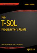
CPU, memory, disk speeds, and network connections have continually increased in speed and capacity since the invention of computers. However, we’re at the point that traditional approaches to making computers run faster are changing due to the economics of the cost of memory versus the speed of CPU processing. In 1965, Gordon E Moore “made the observation that, over the history of computing hardware, the number of transistors in a dense integrated circuit doubles approximately every two years.”1 Since then, this statement has been known as Moore’s Law. Figure 6-1 shows a graph of the increase in the number of transistors on a single circuit.
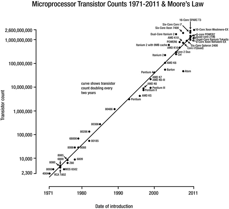
Figure 6-1. Moore’s Law transistor counts
Manufacturers of memory, pixels on a screen, network bandwidth, CPU architecture, and so on have all used Moore’s Law as a guide for long-term planning. It’s hard to believe, but today, increasing the amount of power to a transistor, for faster CPU clock speed, no longer makes economic sense. As the amount of power being sent to a transistor is increased, the transistor heats up to the point that the physical components begin to melt and malfunction. We’ve essentially hit a practical limitation on the clock speed for an individual chip, because it isn’t possible to effectively control the temperature of a CPU. The best way to continue to increase the power of a CPU with the same clock speed is via additional cores per socket.
In parallel to the limitations of CPUs, the cost of memory has continued to decline significantly over time. It’s common for servers and commodity hardware to come equipped with more memory than multimillion-dollar servers had available 20 years ago. Table 6-1 shows the historical price of 1 gigabyte of memory.
Table 6-1. Price of RAM over time2
|
Historic RAM Prices | |
|---|---|
|
Year |
Average Cost per Gigabyte |
|
1980 |
$6,635,520.00 |
|
1985 |
$ 901,120.00 |
|
1990 |
$ 108,544.00 |
|
1995 |
$ 31,641.60 |
|
2000 |
$ 1,149.95 |
|
2005 |
$ 189.44 |
|
2010 |
$ 12.50 |
|
2014 |
$ 9.34 |
In order to make effective use of additional cores and the increase in memory available with modern hardware, software has to be written to take advantage of these hardware trends. The SQL Server 2014 In-Memory features are the result of these trends and customer demand for additional capacity on OLTP databases.
Getting Started with In-Memory Objects
SQL Server 2014 In-Memory features are offered in Enterprise, Developer, and Evaluation (64-bit only) Editions of the software. These features were previously available only to corporations that had a very large budget to spend on specialized software and hardware. Given the way Microsoft has deployed these features in existing editions, you may be able to use them an existing installation of your OLTP database system.
The in-memory objects require a FILESTREAM data file (container) to be created using a memory-optimized data filegroup. From here on, this chapter uses the term container rather than data file; it’s more appropriate because a data file is created on disk at the time data is written to the new memory-optimized tables. Several checkpoint files are created in the memory-optimized data filegroup for the purposes of keeping track of changes to data in the FILESTREAM container file. The data for memory-optimized tables is stored in a combination of the transaction log and checkpoint files until a background thread called an offline checkpoint appends the information to data and delta files. In the event of a server crash or availability group failover, all durable table data is recovered from a combination of the data, delta, transaction log, and checkpoint files. All nondurable tables are re-created, because the schema is durable, but the data is lost. The differences between durable and non-durable tables, advantages, disadvantages, and some use cases are explained further in the section “Step 3,” later in this chapter.
You can alter any existing database or new database to accommodate in-memory data files (containers) by adding the new data and filegroup structures. Several considerations should be taken into account prior to doing so. The following sections cover the steps listed in the code format and SQL Server Management Studio to create these structures.
Step 1: Add a New Memory-Optimized Data FILEGROUP
Typically, before you can begin to using FILESTREAM in SQL Server, you must enable FILESTREAM on the instance of the SQL Server Database Engine. With memory-optimized filegroups, you don’t need to enable FILESTREAM because the mapping to it’s handled by the In-Memory OLTP engine.
The memory-optimized data filegroup should be created on a solid state drive (SSD) or fast serial attached SCSI (SAS) drive. Memory-optimized tables have different access patterns than traditional disk-based tables and require the faster disk subsystems to fully realize the speed benefit of this filegroup. Listing 6-1, adds a new memory-optimized filegroup to our existing AdventureWorks2014 database. This syntax can be used against any existing 2014 database on the proper SQL Server edition of the software.
Listing 6-1. Adding a New Filegroup
IF NOT EXISTS
  (SELECT * FROM AdventureWorks2014.sys.data_spaces WHERE TYPE = 'FX')
ALTER DATABASE AdventureWorks2014
  ADD FILEGROUP [AdventureWorks2014_mem] CONTAINS MEMORY_OPTIMIZED_DATA
GO
This adds an empty memory-optimized data filegroup to which you’ll add containers in the next step. The key words in the syntax are CONTAINS MEMORY_OPTIMIZED_DATA, to create as a memory-optimized data filegroup. You can create multiple containers but only one memory-optimized data filegroup. Adding additional memory-optimized data filegroups results in the following error:
Msg 10797, Level 15, State 2, Line 2
Only one MEMORY_OPTIMIZED_DATA filegroup is allowed per database.
In Listing 6-1, we added a new memory-optimized filegroup using T-SQL code. In the following example, we will do the same using SQL Server Management Studio. Following are the steps to accomplish adding the filegroup via Management Studio (see Figure 6-2):
- Right-click the database to which you want to add the new filegroup, and select Properties.
- Select the Filegroups option, and type in the name of the memory-optimized data filegroup you wish to add.
- Click the Add Filegroup button.

Figure 6-2. Adding a new memory-optimized data filegroup
![]() Note Memory-optimized data filegroups can only be removed by dropping the database. Therefore, you should careful consider the decision to move forward with this architecture.
Note Memory-optimized data filegroups can only be removed by dropping the database. Therefore, you should careful consider the decision to move forward with this architecture.
Step 2: Add a New Memory-Optimized Container
In step-2 we will add a new memory-optimized container. Listing 6-2 shows an example of how this is accomplished using T-SQL code. This code can be used against any database that has a memory-optimized filegroup.
Listing 6-2. Adding a New Container to the Database
IF NOT EXISTS
  ( SELECT * FROM AdventureWorks2014.sys.data_spaces ds
             JOIN AdventureWorks2014.sys.database_files df ON
                  ds.data_space_id=df.data_space_id
            WHERE ds.type='FX'    )
   ALTER DATABASE AdventureWorks2014
       ADD FILE (name=' AdventureWorks2014_mem',
                   filename='C:SQLDataAdventureWorks2014_mem')
      TO FILEGROUP [AdventureWorks2014_mem]
GO
In Listing 6-2, we added a new memory-optimized container to our database using T-SQL code. In the following steps we will do the same using Management Studio. In order to accomplish this, follow the steps outlined below (see Figure 6-3):
- Right-click the database to which you want to add the new container, and select Properties.
- Select the Files option, and type in the name of the file you wish to add.
- Select FILESTREAM Data from the File Type list, and click the Add button.

Figure 6-3. Adding a new filestream container file to a memory-optimized filegroup
It is a best practice to adjust the Autogrowth / Maxsize of a fiegroup; this option is to the right of the "Filegroup" column in Figure 6-4. For a memory-optimized filegroup, you will not be able to adjust this option when creating the fielgroup through Management Studio. This filegroup lives in memory; therefore, the previous practice of altering this option no longer applies. Leave the Autogrowth / Maxsize option set to Unlimited. It’s a limitation of the current version that you can’t specify a MAXSIZE for the specific container you’re creating.
You now have a container in the memory-optimized data filegroup that you previously added to the database. Durable tables save their data to disk in the containers you just defined; therefore, it’s recommended that you create multiple containers across multiple disks, if they’re available to you. SSDs won’t necessarily help performance, because data is accessed in a sequential manner and not in a random-access pattern. The only requirement is that you have performant disks so the data can be accessed efficiently from disk. Multiple disks allow SQL Server to recover data in parallel in the event of a system crash or availability group failover. Your in-memory tables won’t become available until SQL Server has recovered the data into memory.
![]() Note Data and delta file pairs can’t be moved to other containers in the memory-optimized filegroup.
Note Data and delta file pairs can’t be moved to other containers in the memory-optimized filegroup.
Step 3: Create Your New Memory-Optimized Table
Step 1 and Step 2 laid out the foundation necessary to add memory-optimized objects. Listing 6-3 creates a table that in memory. The result is a compiled table with data that resides in memory.
Listing 6-3. Creating a New Memory-Optimized Table
USE AdventureWorks2014;
GO

CREATE SCHEMA [MOD] AUTHORIZATION [dbo];
GO

CREATE TABLE [MOD].[Address]
 (
       AddressID INT NOT NULL IDENTITY(1,1)
    , AddressLine1 NVARCHAR(120) COLLATE Latin1_General_100_BIN2 NOT NULL
    , AddressLine2 NVARCHAR(120) NULL
    , City NVARCHAR(60) COLLATE Latin1_General_100_BIN2 NOT NULL
    , StateProvinceID INT NOT NULL
    , PostalCode NVARCHAR(30) COLLATE Latin1_General_100_BIN2 NOT NULL
    , rowguid UNIQUEIDENTIFIER NOT NULL
                 INDEX [AK_MODAddress_rowguid] NONCLUSTERED
                 CONSTRAINT [DF_MODAddress_rowguid] DEFAULT (NEWID())
    , ModifiedDate DATETIME NOT NULL
            INDEX [IX_MODAddress_ModifiedDate] NONCLUSTERED
                 CONSTRAINT [DF_MODAddress_ModifiedDate] DEFAULT (GETDATE())

    , INDEX [IX_MODAddress_AddressLine1_ City_StateProvinceID_PostalCode]
        NONCLUSTERED
    ( [AddressLine1] ASC, [StateProvinceID] ASC, [PostalCode] ASC )

       , INDEX [IX_MODAddress_City]
       ( [City] DESC )

    , INDEX [IX_MODAddress_StateProvinceID]
        NONCLUSTERED
    ( [StateProvinceID] ASC)

    , CONSTRAINT PK_MODAddress_Address_ID
             PRIMARY KEY NONCLUSTERED HASH
    ( [AddressID]) WITH (BUCKET_COUNT=30000)

) WITH(MEMORY_OPTIMIZED=ON, DURABILITY=SCHEMA_AND_DATA);
GO
![]() Note You don’t need to specify a filegroup when you create an in-memory table. You’re limited to a single memory-optimized filegroup; therefore, SQL Server knows the filegroup to which to add this table.
Note You don’t need to specify a filegroup when you create an in-memory table. You’re limited to a single memory-optimized filegroup; therefore, SQL Server knows the filegroup to which to add this table.
The sample table used for this memory-optimized table example is similar to the AdventureWorks2014.Person.Address table, with several differences:
- The hint at the end of the CREATE TABLE statement is extremely important:
WITH(MEMORY_OPTIMIZED=ON, DURABILITY=SCHEMA_AND_DATA);
- The option MEMORY_OPTIMIZED=ON tells SQL Server that this is a memory-optimized table.
- The DURABILITY=SCHEMA_AND_DATA option defines whether this table will be durable (data recoverable) or non-durable (schema-only recovery) after a server restart. If the durability option isn’t specified, it defaults to SCHEMA_AND_DATA.
- PRIMARY KEY is NONCLUSTERED, because data isn’t physically sorted:
, CONSTRAINT PK_MODAddress_Address_ID
PRIMARY KEY NONCLUSTERED HASH
( [AddressID] ) WITH (BUCKET_COUNT=30000) - The NONCLUSTERED hint is required on a PRIMARY KEY constraint, because SQL Server attempts to create it as a CLUSTERED index by default. Because CLUSTERED indexes aren’t allowed, not specifying the index type results in an error. Additionally, you can’t add a sort hint on the column being used in this index, because HASH indexes can’t be defined in a specific sort order.
- All character string data that is used in an index must use BIN2 collation:
COLLATE Latin1_General_100_BIN2
- Notice that the MOD.Address table purposely doesn’t declare BIN2 collation for the AddressLine2 column, because it isn’t used in an index. Figure 6-8 shows the effect that BIN2 collation has on data in different collation types.
- If you compare the MOD.Address table to Person.Address, you see that the column SpatialLocation is missing. In-memory tables don’t support LOB objects. The SpatialLocation column in Person.Address is defined as a GEOGRAPHY data type, which isn’t supported for memory-optimized tables. If you were converting this data type to be used in a memory-optimized table, you would potentially need to make coding changes to accommodate the lack of the data type.
- The index type HASH with the hint WITH (BUCKET_COUNT=30000) is new. This is discussed further in the “In-Memory OLTP Table Indexes” section of this chapter.
Listing 6-3 added a memory-optimized table using T-SQL. We will now add add a memory-optimized table using Management Studio. Right-click the Tables folder, and select New ![]() Memory-Optimized Table (see Figure 6-4). A new query window opens with the In-Memory Table Creation template script available.
Memory-Optimized Table (see Figure 6-4). A new query window opens with the In-Memory Table Creation template script available.

Figure 6-4. Creating a new memory-optimized table
You now have a very basic working database and table and can begin using the In-Memory features. You can access the table and different index properties using a system view (see Listing 6-4 and Figure 6-5) or Management Studio (see Figure 6-6).
Listing 6-4. Selecting Table Properties from a System View
SELECT t.name as 'Table Name'
    , t.object_id
       , t.schema_id
    , filestream_data_space_id
    , is_memory_optimized
    , durability
    , durability_desc
  FROM sys.tables t
 WHERE type='U'
   AND t.schema_id = SCHEMA_ID(N'MOD'),

Figure 6-5. System view showing MOD.Address table properties
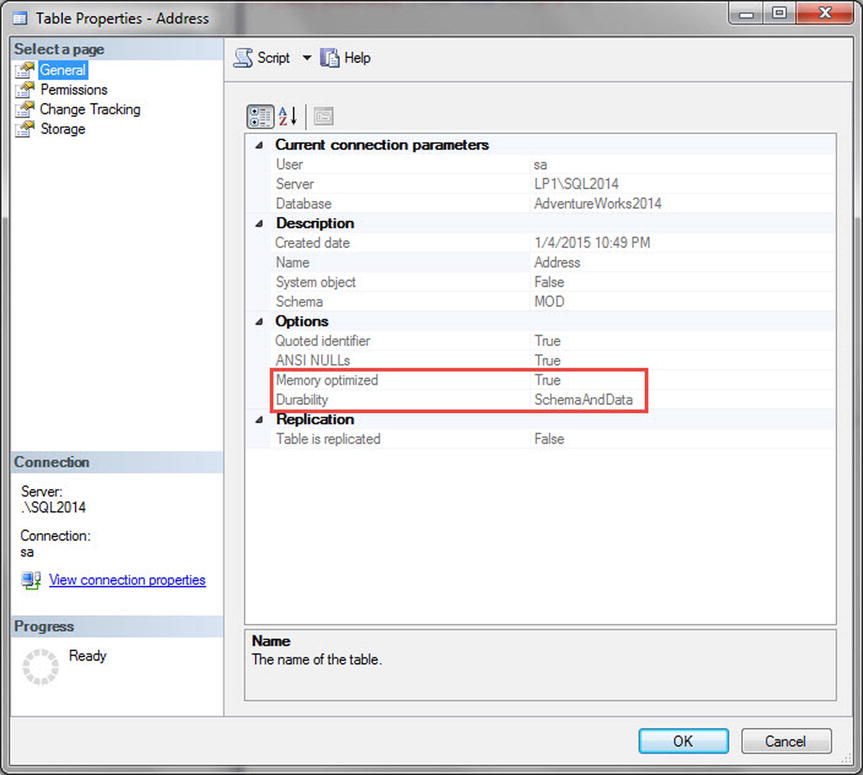
Figure 6-6. Management Studio showing MOD.Address table properties
Now that you’ve configured your database and created a new table, let’s look at an example of the data in this table and some specific issues you may encounter. First you must load the data in the newly created memory-optimized table [MOD].[Address], as shown in Listing 6-5.
Listing 6-5. Inserting Data into the Newly Created Table
SET IDENTITY_INSERT [MOD].[Address] ON;

 INSERT INTO [MOD].[Address]
 (    AddressID, AddressLine1, AddressLine2
       , City, StateProvinceID, PostalCode
    --, SpatialLocation
    , rowguid, ModifiedDate  )

 SELECT AddressID, AddressLine1, AddressLine2
    , City, StateProvinceID, PostalCode
    --, SpatialLocation
    , rowguid, ModifiedDate
   FROM [Person].[Address];

   SET IDENTITY_INSERT [MOD].[Address] OFF;

   UPDATE STATISTICS [MOD].[Address] WITH FULLSCAN, NORECOMPUTE;
   GO
![]() Note In-memory tables don’t support statistics auto-updates. In Listing 6-5, you manually update the statistics after inserting new data.
Note In-memory tables don’t support statistics auto-updates. In Listing 6-5, you manually update the statistics after inserting new data.
Because AddressLine1 is being used in an index on the table, you have to declare the column with a BIN2 collation. The limitation with this collation is that all uppercase AddressLine1 values are sorted before lowercase string values (Z sorts before a). In addition, string comparisons of BIN2 columns don’t give correct results. A lowercase value doesn’t equal an uppercase value when selecting data (A != a). Listing 6-6 gives an example query of the string-comparison scenario.
Listing 6-6. Selecting Data from the AddressLine1 Column
SELECT AddressID, AddressLine1, RowGuid
   FROM [MOD].[Address]
  WHERE AddressID IN (804, 831)
    AND AddressLine1 LIKE '%plaza'
This query correctly results in only one record. However, you would expect two records to be returned, using disk-based tables. Pay careful attention in this area when you’re considering moving your disk-based tables to memory-optimized tables. Figure 6-7 displays the result of the query.

Figure 6-7. AddressLine1 results with no collation
When the collation for the column is altered with a hint (Listing 6-7), the query correctly returns two records (Figure 6-8).
Listing 6-7. Selecting Data from the AddressLine1 Column with Collation
SELECT AddressID, AddressLine1, RowGuid
   FROM [MOD].[Address]
  WHERE AddressID IN (804, 831)
    AND AddressLine1 COLLATE SQL_Latin1_General_CP1_CI_AS LIKE '%plaza';

Figure 6-8. AddressLine1 results with collation
In order to ensure proper results and behavior, you need to specify the collation for all string type columns, with BIN2 collation for comparison and sort operations.
Limitations on Memory-Optimized Tables
When you create a table, you need to take several limitations into account. Following are some of the more common restrictions that you may encounter:
- None of the LOB data types can be used to declare a column (XML, CLR, spatial data types, or any of the MAX data types).
- All the row lengths in a table are limited to 8,060 bytes. This limit is enforced at the time the table is initially created. Disk-based tables allow you to create tables that could potentially exceed 8,060 bytes per row.
- All in-memory tables must have at least one index defined. No heap tables are allowed.
- No DDL/DML triggers are allowed.
- No schema changes are allowed (ALTER TABLE). To change the schema of the table, you would need to drop and re-create the table.
- Partitioning or compressing a memory-optimized table isn’t allowed.
- When you use an IDENTITY column property, it must be initialized to start at 1 and increment by 1.
- If you’re creating a durable table, you must define a primary key constraint.
![]() Note For a comprehensive and up-to-date list of limitations, visit http://msdn.microsoft.com/en-us/library/dn246937.aspx.
Note For a comprehensive and up-to-date list of limitations, visit http://msdn.microsoft.com/en-us/library/dn246937.aspx.
Indexes are used to more efficiently access data stored in tables. Both in-memory tables and disk-based tables benefit from indexes; however, In-Memory OLTP table indexes have some significant differences from their disk-based counterparts. Two types of indexes differ from those of disk-based tables: nonclustered hashes and nonclustered range indexes. These indexes are both contained in memory and are optimized for memory-optimized tables. The differences between in-memory and disk-based table indexes are outlined in Table 6-2.
Table 6-2. Comparison of in-memory and disk-based indexes
|
In-Memory Table |
Disk-Based Table |
|---|---|
|
Must have at least one index |
No indexes required |
|
Clustered Index not allowed; Only hash or range non-clustered indexes allowed. |
Clustered Index usually recommended |
|
Indexes added only at table creation |
Indexes can be added to the table after table creation |
|
No auto update statistics |
Auto update statistics allowed |
|
In-memory table indexes only exist in memory |
Indexes persist on disk and the transaction log |
|
Indexes are created during table creation or database startup |
Indexes are persisted to disk; therefore, they are not rebuilt and can be read from disk |
|
Indexes are covering, since the index contains a memory pointer to the actual row of the data |
Indexes are not covering by default. |
|
There is a limitation of 8 indexes per table |
1 Clustered Index+999 NonClustered=1000 Indexes or 249 XML Indexes |
![]() Note Durable memory-optimized tables require a primary key. By default, a primary key attempts to create a clustered index, which will generate an error for a memory-optimized table. You must specifically indicate NONCLUSTERED as the index type.
Note Durable memory-optimized tables require a primary key. By default, a primary key attempts to create a clustered index, which will generate an error for a memory-optimized table. You must specifically indicate NONCLUSTERED as the index type.
The need for at least one index stems from the architecture of an in-memory table. The table uses index pointers as the only method of linking rows in memory into a table. This is also why clustered indexes aren’t needed on memory-optimized tables; the data isn’t specifically ordered or arranged in any manner.
A new feature of SQL Server 2014 is that you can create indexes inline with the table create statement. Earlier, notice that Listing 6-3 creates an inline nonclustered index with table create:
, rowguid UNIQUEIDENTIFIER NOT NULL
             INDEX [AK_MODAddress_rowguid] NONCLUSTERED
             CONSTRAINT [DF_MODAddress_rowguid] DEFAULT (NEWID())
Inline index creation is new to SQL Server 2014 but not unique to memory-optimized tables. It’s also valid for disk-based tables.
Both hash and range indexes are allowed on the same column. This can be a good strategy when the use cases vary for how the data is accessed.
Hash Indexes
A hash index is an efficient mechanism that accepts input values into a hashing function and maps to a hash bucket. The hash bucket is an array that contains pointers to efficiently return a row of data. The collection of pointers in the hash bucket is the hash index. When created, this index exists entirely in memory.
Hash indexes are best used for single-item lookups, a WHERE clause with an =, or equality joins. They can’t be used for range lookups such as LIKE operations or between queries. The optimizer won’t give you an error, but it isn’t an efficient way of accessing the data. When creating the hash index, you must decide at table-creation time how many buckets to assign for the index. It’s recommended that it should be created at 1.5 to 2 times larger than the existing unique key counts in your table. This is an important assessment, because the bucket count can’t be extended by re-creating the index and the table. The performance of the point lookups doesn’t degrade if you have a bucket count that is larger than necessary. However, performance will suffer if the bucket count is too small. Listing 6-3 used a hash bucket count of 30,000, because the number of unique rows in the table is slightly less than 20,000. Here’s the code that defines the constraint with the bucket count:
, CONSTRAINT PK_MODAddress_Address_ID PRIMARY KEY NONCLUSTERED HASH
(    [AddressID] ASC ) WITH (BUCKET_COUNT=30000)
If your use case requires it, you can create a composite index on a hash index. There are some limitations to be aware of if you decide to use a composite index. The hash index will be used only if the point-lookup search is done on both columns in the index. If both columns aren’t used in the search, the result is an index scan or a scan of all the hash buckets. This occurs because the hash function converts the values from both columns into a hash values. Therefore, in a composite hash index, the value of one column never equates to the hash value of two columns:
HASH(<Column1>) <> HASH(<Column1>, <Column2>)
Let’s compare the affect of a hash index on a memory-optimized table versus a disk-based table clustered index.
![]() Warning This applies to the code in Listing 6-8 and several other examples. Do not attempt to run the DBCC commands on a production system, because they can severely affect the performance of your entire instance.
Warning This applies to the code in Listing 6-8 and several other examples. Do not attempt to run the DBCC commands on a production system, because they can severely affect the performance of your entire instance.
Listing 6-8 includes some DBCC commands to flush all cache pages and make sure the comparisons start in a repeatable state with nothing in memory. It’s highly recommended that these types of commands be run only in a non-production environment that won’t affect anyone else on the instance.
Listing 6-8. Point Lookup on a Hash Index vs. Disk-Based Clustered Index
CHECKPOINT
GO
DBCC DROPCLEANBUFFERS
GO
DBCC FREEPROCCACHE
GO

SET STATISTICS IO ON;

SELECT * FROM Person.Address WHERE AddressId = 26007;
SELECT * FROM MOD.Address WHERE AddressId = 26007;
This first example simply looks at what happens when you compare performance when doing a simple point lookup for a specific value. Both the disk-based table (Person.Address) and the memory-optimized table (MOD.Address) have a clustered and hash index on the AddressID column. The result of running the entire batch is as shown in Figure 6-9 in the Messages tab.

Figure 6-9. Hash index vs. clustered index IO statistics
There are two piece of information worth noting. The first batch to run was the disk-based table, which resulted in two logical reads and two physical reads. The second batch was the memory-optimized table, which didn’t register any logical or physical IO reads because this table’s data and indexes are completely held in memory.
Figure 6-10 clearly shows that the disk-based table took 99% of the entire batch execution time; the memory-optimized table took 1% of the time relative to the entire batch. Both query plans are exactly the same; however, this illustrates the significant difference that a memory-optimized table can make to the simplest of queries.

Figure 6-10. Hash index vs. clustered index point lookup execution plan
Hovering over the Index Seek operator in the execution plan shows a couple of differences. The first is that the Storage category now differentiates between the disk-based table as RowStore and the memory-optimized table as MemoryOptimized. There is also a significant difference between the estimated row size of the two tables.
Next let’s experiment with running a range lookup against the disk-based table and the memory-optimized table. Listing 6-9 does a simple range lookup against the primary key of the table to demonstrate some of the difference in performance (see Figure 6-11).
Listing 6-9. Range Lookup Using a Hash Index
SELECT * FROM PERSON.ADDRESS WHERE ADDRESSID BETWEEN 100 AND 26007;
SELECT * FROM MOD.ADDRESS WHERE ADDRESSID BETWEEN 100 AND 26007;
Figure 6-11. Hash index vs. clustered index range lookup execution plan
This example clearly displays that a memory-optimized table hash index isn’t necessarily quicker than a disk-based clustered index for all use cases. The memory-optimized table had to perform an index scan and then filter the results for the specific criteria you’re looking to get back. The disk-based table clustered index seek is still more efficient for this particular use case. The moral of the story is that it always depends. You should always run through several use cases and determine the best method of accessing your data.
A range index might best be defined as a memory-optimized nonclustered index. When created, this index exists entirely in memory. The memory-optimized nonclustered index works similarly to a disk-based nonclustered index, but it has some significant architectural differences. The architecture for range indexes is based on a new data structure called a Bw-tree.3 The Bw-tree architecture is a latch-free architecture that can take advantage of modern processor caches and multicore chips.
Memory-optimized nonclustered indexes are best used for range-type queries such as (<,>,IN), (All sales orders between dates), and so on. These indexes also work with point lookups but aren’t as optimized for those types of lookups as a hash index. Memory-optimized nonclustered indexes should also be considered over hash indexes when you’re migrating a disk-based table that has a considerable number of duplicate values in a column. The size of the index grows with the size of the data, similar to B-tree disk-based table structures.
When you’re using memory-optimized nonclustered indexes, a handful of limitations and differences from disk-based nonclustered indexes are worth mentioning. Listing 6-3 created the nonclustered index on the City column. Below is an excerpt from the listing, that displays the creation of the nonclustered index.
INDEX [IX_MODAddress_City]
( [City] DESC)
- All the columns that are part of an index must be defined as NOT NULL.
- If the column is defined as a string data type, it must be defined using a BIN2 collation.
- The NONCLUSTERED hint is optional unless the column is the primary key for the table, because SQL Server will try to define a primary key constraint as clustered.
- The sort-order hint on a column in a range index is especially important for a memory-optimized table. SQL Server can’t perform a seek on the index if the order in which the records are accessed is different from the order in which the index was originally defined, which would result in an index scan.
Following are a couple of examples that demonstrate the comparison of a disk-based nonclustered index and a memory-optimized nonclustered index (range index). The two queries in Listing 6-10 select all columns from the Address disk-based table and the memory-optimized table using a single-point lookup of the date. The result of the queries is displayed in Figure 6-12.
Listing 6-10. Single-Point Lookup Using a Range Index
CHECKPOINT
GO
DBCC DROPCLEANBUFFERS
GO
DBCC FREEPROCCACHE
GO

SET STATISTICS IO ON

SELECT * FROM [Person].[Address] WHERE ModifiedDate = '2013-12-21';
SELECT * FROM [MOD].[Address] WHERE ModifiedDate = '2013-12-21';
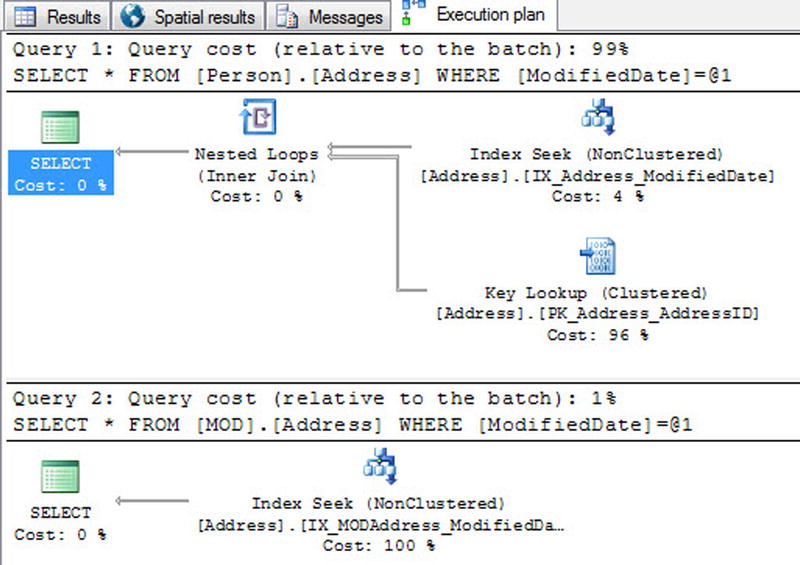
Figure 6-12. Single-point lookup using a nonclustered index comparison
This example displays a significant difference between Query 1 (disk-based table) and Query 2 (memory-optimized index). Both queries use an index seek to get to the row in the table, but the disk-based table has to do an additional key-lookup operation on the clustered index. Because the query is asking for all the columns of data in the row, the disk-based nonclustered index must obtain the pointer to the data through the clustered index. The memory-optimized index doesn’t have the added cost of the key lookup, because all the indexes are covering and, therefore, the index already has a pointer to the additional columns of data.
Next, Listing 6-11 does a range lookup on the disk-based table nonclustered index and a range lookup on the memory-optimized nonclustered index. The difference between the two queries is displayed in Figure 6-13.
Listing 6-11. Range Lookup Using a Range Index
CHECKPOINT
GO
DBCC DROPCLEANBUFFERS
GO
DBCC FREEPROCCACHE
GO

SET STATISTICS IO ON

SELECT * FROM [Person].[Address] WHERE ModifiedDate
              BETWEEN '2013-12-01' AND '2013-12-21';
SELECT * FROM [MOD].[Address] WHERE ModifiedDate
              BETWEEN '2013-12-01' AND '2013-12-21';

Figure 6-13. Range Lookup Comparison
The results are as expected. The memory-optimized nonclustered index performs significantly better than the disk-based nonclustered index when performing a range query using a range index.
Natively Compiled Stored Procedures
Natively compile stored procedures are similar in purpose to disk-based stored procedures, with the major difference that a natively compiled stored procedure is compiled into C and then into machine language stored as a DLL. The DLL allows SQL Server to access the stored-procedure code more quickly, to take advantage of parallel processing and significant improvements in execution. There are several limitations, but if used correctly, natively compiled stored procedures can yield a 2x or more increase in performance.
To get started, let’s examine the outline of a natively compiled stored procedure in Listing 6-12 in detail.
Listing 6-12. Natively Compiled Stored Procedure Example
1 CREATE PROCEDURE selAddressModifiedDate
2 (    @BeginModifiedDate DATETIME
3     , @EndmodifiedDate DATETIME )
4  WITH
5    NATIVE_COMPILATION
6    , SCHEMABINDING
7    , EXECUTE AS OWNER
8  AS
9  BEGIN ATOMIC
10  WITH
11 ( TRANSACTION ISOLATION LEVEL = SNAPSHOT
12      LANGUAGE = N'us_english')
13
14  -- T-SQL Logic Here
15  SELECT AddressID, AddressLine1
16        , AddressLine2, City
17        , StateProvinceID, PostalCode
18        , rowguid, ModifiedDate
19    FROM [MOD].[Address]
20   WHERE ModifiedDate
21         BETWEEN @BeginModifiedDate AND @EndmodifiedDate;
22
23  END;
The requirements to create a natively compiled stored procedure are as follows:
- Line 5, NATIVE COMPILATION: This option tells SQL Server that the procedure is to be compiled into a DLL. If you add this option, you must also specify the SCHEMABINDING, EXECUTE AS, and BEGIN ATOMIC options.
- Line 6, SCHEMABINDING: This option binds the stored procedure to the schema of the objects it references. At the time the stored procedure is compiled, the schema and of the objects it references are compiled into the DLL. When the procedure is executed, it doesn’t have to check to see whether the columns of the objects it references have been altered. This offers the fastest and shortest method of executing a stored procedure. If any of the underlying objects it references are altered, you’re first forced to drop and recompile the stored procedure with any changes to the underlying objects it references.
- Line 7, EXECUTE AS OWNER: The default execution context for a stored procedure is EXECUTE AS CALLER. Natively compiled stored procedures don’t support this caller context and must be specified as one of the options EXECUTE AS OWNER, SELF, or USER. This is required so that SQL Server doesn’t have to check execution rights for the user every time they attempt to execute the stored procedure. The execution rights are hardcoded and compiled into the DLL to optimize the speed of execution.
- Line 9, BEGIN ATOMIC: Natively compiled stored procedures have the requirement that the body must consist of exactly one atomic block. The atomic block is part of the ANSI SQL standard that specifies that either the entire stored procedure succeeds or the entire stored procedure logic fails and rolls back as a whole. At the time the stored procedure is called, if an existing transaction is open, the stored procedure joins the transaction and commits. If no transaction is open, then the stored procedure creates its own transaction and commits.
- Lines 11 and 12, TRANSACTION ISOLATION: All the session settings are fixed at the time the stored procedure is created. This is done to optimize the stored procedure’s performance at execution time.
Those are the main options in a natively compiled stored procedure that are unique to its syntax, versus a disk-based stored procedure. There are a significant number of limitations when creating a natively compiled stored procedure. Some of the more common limitations are listed next:
- Objects must be called using two-part names (schema.table).
- Temporary tables from tempdb can’t be used and should be replaced with table variables or nondurable memory-optimized tables.
- A natively compiled stored procedure can’t be accessed from a distributed transaction.
- The stored procedure can’t access disk-based tables, only memory-optimized tables.
- The stored procedure can’t use any of the ranking functions.
- DISTINCT in a query isn’t supported.
- EXISTS or IN are not supported functions.
- Common table expressions (CTEs) are not supported constructs.
- Subqueries aren’t available.
![]() Note For a comprehensive list of limitations, visit http://msdn.microsoft.com/en-us/library/dn246937.aspx.
Note For a comprehensive list of limitations, visit http://msdn.microsoft.com/en-us/library/dn246937.aspx.
Execution plans for queries in the procedure are optimized when the procedure is compiled. This happens only when the procedure is created and when the server restarts, not when statistics are updated. Therefore, the tables need to contain a representative set of data, and statistics need to be up-to-date before the procedures are created. (Natively compiled stored procedures are recompiled if the database is taken offline and brought back online.)
EXERCISES
- Which editions of SQL Server support the new In-Memory features?
- Developer Edition
- Enterprise Edition
- Business Intelligence Edition
- All of the above
- When defining a string type column in an in-memory table, you must always use a BIN2 collation.
[True / False]
- You want to define the best index type for a date column in your table. Which index type might be best suited for this column, if it is being used for reporting purposes using a range of values?
- Hash index
- Clustered index
- Range index
- A and B
- When creating a memory-optimized table, if you do not specify the durability option for the table, it will default to SCHEMA_AND_DATA.
[True / False]
- Memory-optimized tables always require a primary key constraint.
[True / False]
- Natively compiled stored procedures allow for which of the following execution contexts?
- EXECUTE AS OWNER
- EXECUTE AS SELF
- EXECUTE AS USER
- A and B
- A, B, and C
_____________________
1“Moore’s Law,” http://en.wikipedia.org/wiki/Moore's_law.
2“Average Historic Price of RAM,” Statistic Brain, www.statisticbrain.com/average-historic-price-of-ram.
3Justin J. Levandoski, David B. Lomet, and Sudipta Sengupta, “The Bw-Tree: A B-tree for New Hardware Platforms,” Microsoft Research, April 8, 2013, http://research.microsoft.com/apps/pubs/default.aspx?id=178758.