
Chapter 6. Maximizing Speed and Performance of TensorFlow: A Handy Checklist
Life is all about making do with what we have, and optimization is the name of the game.
It’s not about having everything—it’s about using your resources wisely. Maybe we really want to buy that Ferrari, but our budget allows for a Toyota. You know what, though? With the right kinds of performance tuning, we can make that bad boy race at NASCAR!
Let’s look at this in terms of the deep learning world. Google, with its engineering might and TPU pods capable of boiling the ocean, set a speed record by training ImageNet in just about 30 minutes! And yet, just a few months later, a ragtag team of three researchers (Andrew Shaw, Yaroslav Bulatov, and Jeremy Howard), with $40 in their pockets using a public cloud, were able to train ImageNet in only 18 minutes!
The lesson we can draw from these examples is that the amount of resources that you have is not nearly as important as using them to their maximum potential. It’s all about doing more with less. In that spirit, this chapter is meant to serve as a handy checklist of potential performance optimizations that we can make when building all stages of the deep learning pipelines, and will be useful throughout the book. Specifically, we will discuss optimizations related to data preparation, data reading, data augmentation, training, and finally inference.
And the story starts and ends with two words...
GPU Starvation
A commonly asked question by AI practitioners is, “Why is my training so slow?” The answer more often than not is GPU starvation.
GPUs are the lifelines of deep learning. They can also be the most expensive component in a computer system. In light of that, we want to fully utilize them. This means that a GPU should not need to wait for data to be available from other components for processing. Rather, when the GPU is ready to process, the preprocessed data should already be available at its doorstep and ready to go. Yet, the reality is that the CPU, memory, and storage are frequently the performance bottlenecks, resulting in suboptimal utilization of the GPU. In other words, we want the GPU to be the bottleneck, not the other way round.
Buying expensive GPUs for thousands of dollars can be worthwhile, but only if the GPU is the bottleneck to begin with. Otherwise, we might as well burn the cash.
To illustrate this better, consider Figure 6-1. In a deep learning pipeline, the CPU and GPU work in collaboration, passing data to each other. The CPU reads the data, performs preprocessing steps including augmentations, and then passes it on to the GPU for training. Their collaboration is like a relay race, except one of the relay runners is an Olympic athlete, waiting for a high school track runner to pass the baton. The more time the GPU stays idle, the more wasted resources.

Figure 6-1. GPU starvation, while waiting for CPU to finish preparing the data
A large portion of this chapter is devoted to reducing the idle time of the GPU and the CPU.
A logical question to ask is: how do we know whether the GPU is starving? Two handy tools can help us answer this question:
nvidia-smi-
This command shows GPU statistics including utilization.
- TensorFlow Profiler + TensorBoard
-
This visualizes program execution interactively in a timeline within TensorBoard.
nvidia-smi
Short for NVIDIA System Management Interface program, nvidia-smi provides detailed statistics about our precious GPUs, including memory, utilization, temperature, power wattage, and more. It’s a geek’s dream come true.
Let’s take it for a test drive:
$ nvidia-smi
Figure 6-2 shows the result.

Figure 6-2. Terminal output of nvidia-smi highlighting the GPU utilization
While training a network, the key figure we are interested in is the GPU utilization, defined in the documentation as the percent of time over the past second during which one or more kernels was executing on the GPU. Fifty-one percent is frankly not that great. But this is utilization at the moment in time when nvidia-smi is called. How do we continuously monitor these numbers? To better understand the GPU usage, we can refresh the utilization metrics every half a second with the watch command (it’s worth memorizing this command):
$ watch -n .5 nvidia-smi
Note
Although GPU utilization is a good proxy for measuring the efficiency of our pipeline, it does not alone measure how well we’re using the GPU, because the work could still be using a small fraction of the GPU’s resources.
Because staring at the terminal screen with the number jumping around is not the most optimal way to analyze, we can instead poll the GPU utilization every second and dump that into a file. Run this for about 30 seconds while any GPU-related process is running on our system and stop it by pressing Ctrl+C:
$ nvidia-smi --query-gpu=utilization.gpu --format=csv,noheader,nounits -f
gpu_utilization.csv -l 1
Now, calculate the median GPU utilization from the file generated:
$ sort -n gpu_utilization.csv | grep -v '^0$' | datamash median 1
Tip
Datamash is a handy command-line tool that performs basic numeric, textual, and statistical operations on textual data files. You can find instructions to install it at https://www.gnu.org/software/datamash/.
nvidia-smi is the most convenient way to check our GPU utilization on the command line. Could we get a deeper analysis? It turns out, for advanced users, TensorFlow provides a powerful set of tools.
TensorFlow Profiler + TensorBoard
TensorFlow ships with tfprof (Figure 6-3), the TensorFlow profiler to help analyze and understand the training process at a much deeper level, such as generating a detailed model analysis report for each operation in our model. But the command line can be a bit daunting to navigate. Luckily, TensorBoard, a suite of browser-based visualization tools for TensorFlow, includes a plugin for the profiler that lets us interactively debug the network with a few mouse clicks. This includes Trace Viewer, a feature that shows events in a timeline. It helps investigate how resources are being used precisely at a given period of time and spot inefficiencies.
Note
As of this writing, TensorBoard is fully supported only in Google Chrome and might not show the profile view in other browsers, like Firefox.

Figure 6-3. Profiler’s timeline in TensorBoard shows an idle GPU while the CPU is processing as well as CPU idling while the GPU is processing
TensorBoard, by default, has the profiler enabled. Activating TensorBoard involves a simple callback function:
tensorboard_callback=tf.keras.callbacks.TensorBoard(log_dir="/tmp",profile_batch=7)model.fit(train_data,steps_per_epoch=10,epochs=2,callbacks=[tensorboard_callback])
When initializing the callback, unless profile_batch is explicitly specified, it profiles the second batch. Why the second batch? Because the first batch is usually slower than the rest due to some initialization overhead.
Note
It bears reiterating that profiling using TensorBoard is best suited for power users of TensorFlow. If you are just starting out, you are better off using nvidia-smi. (Although nvidia-smi is a far more capable than just providing GPU utilization info, which is typically how most practitioners use it.) For users wanting even deeper access to their hardware utilization metrics, NVIDIA Nsight is a great tool.
Alright. With these tools at our disposal, we know that our program needs some tuning and has room for efficiency improvements. We look at those areas one by one in the next few sections.
How to Use This Checklist
In business, an oft-quoted piece of advice is “You can’t improve what you can’t measure.” This applies to deep learning pipelines, as well. Tuning performance is like a science experiment. You set up a baseline run, tune a knob, measure the effect, and iterate in the direction of improvement. The items on the following checklist are our knobs—some are quick and easy, whereas others are more involved.
To use this checklist effectively, do the following:
-
Isolate the part of the pipeline that you want to improve.
-
Find a relevant point on the checklist.
-
Implement, experiment, and observe if runtime is reduced. If not reduced, ignore change.
-
Repeat steps 1 through 3 until the checklist is exhausted.
Some of the improvements might be minute, some more drastic. But the cumulative effect of all these changes should hopefully result in faster, more efficient execution and best of all, more bang for the buck for your hardware. Let’s look at each area of the deep learning pipeline step by step, including data preparation, data reading, data augmentation, training, and, finally, inference.
Performance Checklist
Data Preparation
Data Augmentation
Training
Inference
Note
A printable version of this checklist is available at http://PracticalDeepLearning.ai. Feel free to use it as a reference next time you train or deploy a model. Or even better, spread the cheer by sharing with your friends, colleagues, and more importantly, your manager.
Data Preparation
There are a few optimizations that we can make even before we do any kind of training, and they have to do with how we prepare our data.
Store as TFRecords
Image datasets typically consist of thousands of tiny files, each file measuring a few kilobytes. And our training pipeline must read each file individually. Doing this thousands of times has significant overhead, causing a slowdown of the training process. That problem is even more severe in the case of spinning hard drives, for which the magnetic head needs to seek to the beginning of each file. This problem is further exacerbated when the files are stored on a remote storage service like the cloud. And there lies our first hurdle!
To speed up the reads, one idea is to combine thousands of files into a handful of larger files. And that’s exactly what TFRecord does. It stores data in efficient Protocol Buffer (protobuf) objects, making them quicker to read. Let’s see how to create TFRecord files:
# Create TFRecord filesimporttensorflowastffromPILimportImageimportnumpyasnpimportiocat="cat.jpg"img_name_to_labels={'cat':0}img_in_string=open(cat,'rb').read()label_for_img=img_name_to_labels['cat']defgetTFRecord(img,label):feature={'label':_int64_feature(label),'image_raw':_bytes_feature(img),}returntf.train.Example(features=tf.train.Features(feature=feature))withtf.compat.v1.python_io.TFRecordWriter('img.tfrecord')aswriter:forfilename,labelinimg_name_to_labels.items():image_string=open(filename,'rb').read()tf_example=getTFRecord(image_string,label)writer.write(tf_example.SerializeToString())
Now, let’s take a look at reading these TFRecord files:
# Reading TFRecord filesdataset=tf.data.TFRecordDataset('img.tfrecord')ground_truth_info={'label':tf.compat.v1.FixedLenFeature([],tf.int64),'image_raw':tf.compat.v1.FixedLenFeature([],tf.string),}defmap_operation(read_data):returntf.compat.v1.parse_single_example(read_data,ground_truth_info)imgs=dataset.map(map_operation)forimage_featuresinimgs:image_raw=image_features['image_raw'].numpy()label=image_features['label'].numpy()image=Image.open(io.BytesIO(image_raw))image.show()(label)
So, why not join all of the data in a single file, like say for ImageNet? Although reading thousands of tiny files harms performance due to the overhead involved, reading gigantic files is an equally bad idea. They reduce our ability to make parallel reads and parallel network calls. The sweet spot to shard (divide) a large dataset in TFRecord files lies at around 100 MB.
Reduce Size of Input Data
Image datasets with large images need to be resized before passing through to the GPU. This means the following:
-
Repeated CPU cycles at every iteration
-
Repeated I/O bandwidth being consumed at a larger rate than needed in our data pipeline
One good strategy to save compute cycles is to perform common preprocessing steps once on the entire dataset (like resizing) and then saving the results in TFRecord files for all future runs.
Use TensorFlow Datasets
For commonly used public datasets, from MNIST (11 MB) to CIFAR-100 (160 MB) all the way to MS COCO (38 GB) and Google Open Images (565 GB), it’s quite an effort to download the data (often spread across multiple zipped files). Imagine your frustration if after downloading 95% of the file slowly, the connection becomes spotty and breaks. This is not unusual because these files are typically hosted on university servers, or are downloaded from various sources like Flickr (as is the case with ImageNet 2012, which gives us the URLs from which to download 150 GB-plus of images). A broken connection might mean having to start all over again.
If you think that was tedious, the real challenge actually begins only after you successfully download the data. For every new dataset, we now need to hunt through the documentation to determine how the data is formatted and organized, so we can begin reading and processing appropriately. Then, we need to split the data into training, validation, and test sets (preferably converting to TFRecords). And when the data is so large as to not fit in memory, we will need to do some manual jiu-jitsu to read it and feed it efficiently to the training pipeline. We never said it was easy.
Alternately, we could skip all the pain by consuming the high-performance, ready-to-use TensorFlow Datasets package. With several famous datasets available, it downloads, splits, and feeds our training pipeline using best practices in a few lines.
Let’s look at which datasets are available.
importtensorflow_datasetsastfds# See available datasets(tfds.list_builders())
===== Output =====
['abstract_reasoning', 'bair_robot_pushing_small', 'caltech101', 'cats_vs_dogs',
'celeb_a', 'celeb_a_hq', 'chexpert', 'cifar10', 'cifar100', 'cifar10_corrupted',
'cnn_dailymail', 'coco2014', 'colorectal_histology',
'colorectal_histology_large', 'cycle_gan' ...
There are more than 100 datasets as of this writing, and that number is steadily increasing. Now, let’s download, extract, and make an efficient pipeline using the training set of CIFAR-10:
train_dataset=tfds.load(name="cifar100",split=tfds.Split.TRAIN)train_dataset=train_dataset.shuffle(2048).batch(64)
That’s it! The first time we execute the code, it will download and cache the dataset on our machine. For every future run, it will skip the network download and directly read from the cache.
Data Reading
Now that the data is prepared, let’s look for opportunities to maximize the throughput of the data reading pipeline.
Use tf.data
We could choose to manually read every file from our dataset with Python’s built-in I/O library. We could simply call open for each file and we’d be good to go, right? The main downside in this approach is that our GPU would be bottlenecked by our file reads. Every time we read a file, the GPU needs to wait. Every time the GPU starts processing its input, we wait before we read the next file from disk. Seems rather wasteful, doesn’t it?
If there’s only one thing you can take away from this chapter, let it be this: tf.data is the way to go for building a high-performance training pipeline. In the next few sections, we explore several aspects of tf.data that you can exploit to improve training speed.
Let’s set up a base pipeline for reading data:
files=tf.data.Dataset.list_files("./training_data/*.tfrecord")dataset=tf.data.TFRecordDataset(files)dataset=dataset.shuffle(2048).repeat().map(lambdaitem:tf.io.parse_single_example(item,features)).map(_resize_image).batch(64)
Prefetch Data
In the pipeline we discussed earlier, the GPU waits for the CPU to generate data, and then the CPU waits for the GPU to finish computation before generating data for the next cycle. This circular dependency causes idle time for both CPU and GPU, which is inefficient.
The prefetch function helps us here by delinking the production of the data (by the CPU) from the consumption of the data (by the GPU). Using a background thread, it allows data to be passed asynchronously into an intermediate buffer, where it is readily available for a GPU to consume. The CPU now carries on with the next computation instead of waiting for the GPU. Similarly, as soon as the GPU is finished with its previous computation, and there’s data readily available in the buffer, it starts processing.
To use it, we can simply call prefetch on our dataset at the very end of our pipeline along with a buffer_size parameter (which is the maximum amount of data that can be stored). Usually buffer_size is a small number; 1 is good enough in many cases:
dataset=dataset.prefetch(buffer_size=16)
In just a few pages, we show you how to find an optimal value for this parameter.
In summary, if there’s an opportunity to overlap CPU and GPU computations, prefetch will automatically exploit it.
Parallelize CPU Processing
It would be a waste to have a CPU with multiple cores but doing all of our processing on only one of them. Why not take advantage of the rest? This is exactly where the num_parallel_calls argument in the map function comes in handy:
dataset=dataset.map(lambdaitem:tf.io.parse_single_example(item,features),num_parallel_calls=4)
This starts multiple threads to parallelize processing of the map() function. Assuming that there is no heavy application running in the background, we will want to set num_parallel_calls to the number of CPU cores on our system. Anything more will potentially degrade the performance due to the overhead of context switching.
Parallelize I/O and Processing
Reading files from disk or worse, over a network, is a huge cause of bottlenecks. We might possess the best CPU and GPU in the world, but if we don’t optimize our file reads, it would all be for naught. One solution that addresses this problem is to parallelize both I/O and subsequent processing (also known as interleaving).
dataset=files.interleave(map_func,num_parallel_calls=4)
In this command, two things are happening:
-
The input data is acquired in parallel (by default equal to the number of cores on the system).
-
On the acquired data, setting the
num_parallel_callsparameter allows themap_funcfunction to execute on multiple parallel threads and read from the incoming data asynchronously.
If num_parallel_calls was not specified, even if the data were read in parallel, map_func would run synchronously on a single thread. As long as map_func runs faster than the rate at which the input data is coming in, there will not be a problem. We definitely want to set num_parallel_calls higher if map_func becomes a bottleneck.
Enable Nondeterministic Ordering
For many datasets, the reading order is not important. After all, we might be randomizing their ordering anyway. By default, when reading files in parallel, tf.data still attempts to produce their outputs in a fixed round-robin order. The disadvantage is that we might encounter a “straggler” along the way (i.e., an operation that takes a lot longer than others, such as a slow file read, and holds up all other operations). It’s like a grocery store line where the person in front of us insists on using cash with the exact change, whereas everyone else uses a credit card. So instead of blocking all the subsequent operations that are ready to give output, we skip over the stragglers until they are done with their processing. This breaks the ordering while reducing wasted cycles waiting for the handful of slower operations:
options=tf.data.Options()options.experimental_deterministic=Falsedataset=tf.data.Dataset.list_files("./training_data/")dataset=dataset.with_options(options)dataset=dataset.interleave(tf.data.TFRecordDataset,num_parallel_calls=4)
Cache Data
The Dataset.cache() function allows us to make a copy of data either in memory or as a file on disk. There are two reasons why you might want to cache a dataset:
-
To avoid repeatedly reading from disk after the first epoch. This is obviously effective only when the cache is in memory and can fit in the available RAM.
-
To avoid having to repeatedly perform expensive CPU operations on data (e.g., resizing large images to a smaller size).
Tip
Cache is best used for data that is not going to change. It is recommended to place cache() before any random augmentations and shuffling; otherwise, caching at the end will result in exactly the same data and order in every run.
Depending on our scenario, we can use one of the two following lines:
dataset=dataset.cache()# in-memorydataset=dataset.cache(filename='tmp.cache')# on-disk
It’s worth noting that in-memory cache is volatile and hence only shows performance improvements in the second epoch of every run. On the other hand, file-based cache will make every run faster (beyond the very first epoch of the first run).
Tip
In the “Reduce Size of Input Data”, we mentioned preprocessing the data and saving it as TFRecord files as input to future data pipelines. Using the cache() function directly after the preprocessing step in your pipeline would give a similar performance with a single word change in code.
Turn on Experimental Optimizations
TensorFlow has many built-in optimizations, often initially experimental and turned off by default. Depending on your use case, you might want to turn on some of them to squeeze out just a little more performance from your pipeline. Many of these optimizations are detailed in the documentation for tf.data.experimental.OptimizationOptions.
Note
Here’s a quick refresher on filter and map operations:
- Filter
-
A filter operation goes through a list element by element and grabs those that match a given condition. The condition is supplied as a lambda operation that returns a boolean value.
- Map
-
A map operation simply takes in an element, performs a computation, and returns an output. For example, resizing an image.
Let’s look at a few experimental optimizations that are available to us, including examples of two consecutive operations that could benefit from being fused together as one single operation.
Filter fusion
Sometimes, we might want to filter based on multiple attributes. Maybe we want to use only images that have both a dog and a cat. Or, in a census dataset, only look at families above a certain income threshold who also live within a certain distance to the city center. filter_fusion can help speed up such scenarios. Consider the following example:
dataset=dataset.filter(lambdax:x<1000).filter(lambdax:x%3==0)
The first filter performs a full pass over the entire dataset and returns elements that are less than 1,000. On this output, the second filter does another pass to further remove elements not divisible by three. Instead of doing two passes over many of the same elements, we could instead combine both the filter operations into one pass using an AND operation. That is precisely what the filter_fusion option enables—combining multiple filter operations into one pass. By default, it is turned off. You can enable it by using the following statement:
options=tf.data.Options()options.experimental_optimization.filter_fusion=Truedataset=dataset.with_options(options)
Map and filter fusion
Consider the following example:
dataset=dataset.map(lambdax:x*x).filter(lambdax:x%2==0)
In this example, the map function does a full pass on the entire dataset to calculate the square of every element. Then, the filter function discards the odd elements. Rather than doing two passes (more so in this particularly wasteful example), we could simply fuse the map and filter operations together by turning on the map_and_filter_fusion option so that they operate as a single unit:
options.experimental_optimization.map_and_filter_fusion=True
Autotune Parameter Values
You might have noticed that many of the code examples in this section have hardcoded values for some of the parameters. For the combination of the problem and hardware at hand, you can tune them for maximum efficiency. How to tune them? One obvious way is to manually tweak the parameters one at a time and isolate and observe the impact of each of them on the overall performance until we get the precise parameter set. But the number of knobs to tune quickly gets out of hand due to the combinatorial explosion. If this wasn’t enough, our finely tuned script wouldn’t necessarily be as efficient on another machine due to differences in hardware such as the number of CPU cores, GPU availability, and so on. And even on the same system, depending on resource usage by other programs, these knobs might need to be adjusted over different runs.
How do we solve this? We do the opposite of manual tuning: autotuning. Using hill-climbing optimization algorithms (which are a type of heuristic-driven search algorithms), this option automatically finds the ideal parameter combination for many of the tf.data function parameters. Simply use tf.data.experimental.AUTOTUNE instead of manually assigning numbers. It’s the one parameter to rule them all. Consider the following example:
dataset=dataset.prefetch(buffer_size=tf.data.experimental.AUTOTUNE)
Isn’t that an elegant solution? We can do that for several other function calls in the tf.data pipeline. The following is an example of combining together several optimizations from the section “Data Reading” to make a high-performance data pipeline:
options=tf.data.Options()options.experimental_deterministic=Falsedataset=tf.data.Dataset.list_files("/path/*.tfrecord")dataset=dataset.with_options(options)dataset=files.interleave(tf.data.TFRecordDataset,num_parallel_calls=tf.data.experimental.AUTOTUNE)dataset=dataset.map(preprocess,num_parallel_calls=tf.data.experimental.AUTOTUNE)dataset=dataset.cache()dataset=dataset.repeat()dataset=dataset.shuffle(2048)dataset=dataset.batch(batch_size=64)dataset=dataset.prefetch(buffer_size=tf.data.experimental.AUTOTUNE)
Data Augmentation
Sometimes, we might not have sufficient data to run our training pipeline. Even if we did, we might still want to manipulate the images to improve the robustness of our model—with the help of data augmentation. Let’s see whether we can make this step any faster.
Use GPU for Augmentation
Data preprocessing pipelines can be elaborate enough that you could write an entire book about them. Image transformation operations such as resizing, cropping, color transformations, blurring, and so on are commonly performed on the data immediately after it’s read from disk into memory. Given that these are all matrix transformation operations, they might do well on a GPU.
OpenCV, Pillow, and the built-in Keras augmentation functionality are the most commonly used libraries in computer vision for working on images. There’s one major limitation here, though. Their image processing is primarily CPU based (although you can compile OpenCV to work with CUDA), which means that the pipeline might not be fully utilizing the underlying hardware to its true potential.
Note
As of August 2019, there are efforts underway to convert Keras image augmentation to be GPU accelerated, as well.
There are a few different GPU-bound options that we can explore.
tf.image built-in augmentations
tf.image provides some handy augmentation functions that we can seamlessly plug into a tf.data pipeline. Some of the methods include image flipping, color augmentations (hue, saturation, brightness, contrast), zooming, and rotation. Consider the following example, which changes the hue of an image:
updated_image=tf.image.adjust_hue(image,delta=0.2)
The downside to relying on tf.image is that the functionality is much more limited compared to OpenCV, Pillow, and even Keras. For example, the built-in function for image rotation in tf.image only supports rotating images by 90 degrees counter-clockwise. If we need to be able to rotate by an arbitrary amount, such as 10 degrees, we’d need to manually build that functionality. Keras, on the other hand, provides that functionality out of the box.
As another alternative to the tf.data pipeline, the NVIDIA Data Loading Library (DALI) offers a fast data loading and preprocessing pipeline accelerated by GPU processing. As shown in Figure 6-4, DALI implements several common steps including resizing an image and augmenting an image in the GPU, immediately before the training. DALI works with multiple deep learning frameworks including TensorFlow, PyTorch, MXNet, and others, offering portability of the preprocessing pipelines.
NVIDIA DALI
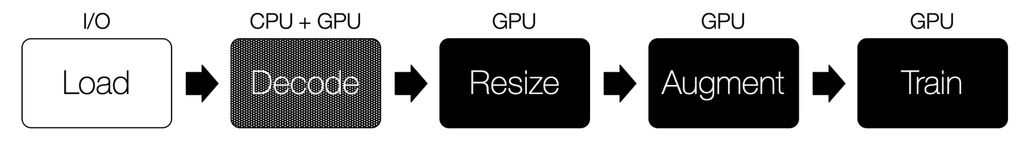
Figure 6-4. The NVIDIA DALI pipeline
Additionally, even JPEG decoding (a relatively heavy task) can partially make use of the GPU, giving it an additional boost. This is done using nvJPEG, a GPU-accelerated library for JPEG decoding. For multi-GPU tasks, this scales near linearly as the number of GPUs increases.
NVIDIAs efforts culminated in a record-breaking MLPerf entry (which benchmarks machine learning hardware, software, and services), training a ResNet-50 model in 80 seconds.
Training
For those beginning their performance optimization journey, the quickest wins come from improving the data pipelines, which is relatively easy. For a training pipeline that is already being fed data fast, let’s investigate optimizations for our actual training step.
Use Automatic Mixed Precision
“One line to make your training two to three times faster!”
Weights in deep learning models are typically stored in single-precision; that is, 32-bit floating point, or as it’s more commonly referenced: FP32. Putting these models in memory-constrained devices such as mobile phones can be challenging to accommodate. A simple trick to make models smaller is to convert them from single-precision (FP32) to half-precision (FP16). Sure, the representative power of these weights goes down, but as we demonstrate later in this chapter (“Quantize the Model”), neural networks are resilient to small changes, much like they are resilient to noise in images. Hence, we get the benefits of a more efficient model without sacrificing much accuracy. In fact, we can even reduce the representation to 8-bit integers (INT8) without a significant loss in accuracy, as we will see in some upcoming chapters.
So, if we can use reduced-precision representation during inference, could we do the same during training, as well? Going from 32-bit to 16-bit representation would effectively mean double the memory bandwidth available, double the model size, or double the batch size can be accommodated. Unfortunately, it turns out that using FP16 naïvely during training can potentially lead to a significant loss in model accuracy and might not even converge to an optimal solution. This happens because of FP16’s limited range for representing numbers. Due to a lack of adequate precision, any updates to the model during training, if sufficiently small, will cause an update to not even register. Imagine adding 0.00006 to a weight value of 1.1. With FP32, the weight would be correctly updated to 1.10006. With FP16, however, the weight would remain 1.1. Conversely, any activations from layers such as Rectified Linear Unit (ReLU) could be high enough for FP16 to overflow and hit infinity (NaN in Python).
The easy answer to these challenges is to use automatic mixed-precision training. In this method, we store the model in FP32 as a master copy and perform the forward/backward passes of training in FP16. After each training step is performed, the final update from that step is then scaled back up to FP32 before it is applied to the master copy. This helps avoid the pitfalls of FP16 arithmetic and results in a lower memory footprint, and faster training (experiments have shown increases in speed by two to three times), while achieving similar accuracy levels as training solely in FP32. It is noteworthy that newer GPU architectures like the NVIDIA Volta and Turing especially optimize FP16 operations.
To enable mixed precision during training, we simply need to add the following line to the beginning of our Python script:
os.environ['TF_ENABLE_AUTO_MIXED_PRECISION'] = '1'
Use Larger Batch Size
Instead of using the entire dataset for training in one batch, we train with several minibatches of data. This is done for two reasons:
-
Our full data (single batch) might not fit in the GPU RAM.
-
We can achieve similar training accuracy by feeding many smaller batches, just as you would by feeding fewer larger batches.
Having smaller minibatches might not fully utilize the available GPU memory, so it’s vital to experiment with this parameter, see its effect on the GPU utilization (using the nvidia-smi command), and choose the batch size that maximizes the utilization. Consumer GPUs like the NVIDIA 2080 Ti ship with 11 GB of GPU memory, which is plenty for efficient models like MobileNet family.
For example on hardware with the 2080 Ti graphics card, using 224 x 224 resolution images and MobileNetV2 model, the GPU can accommodate a batch size up to 864. Figure 6-5 shows the effect of varying batch sizes from 4 to 864, on both the GPU utilization (solid line) as well as the time per epoch (dashed line). As we can see in the figure, the higher the batch size, the higher the GPU utilization, leading to a shorter training time per epoch.
Even at our max batch size of 864 (before running out of memory allocation), the GPU utilization does not cross 85%. This means that the GPU was fast enough to handle the computations of our otherwise very efficient data pipeline. Replacing MobileNetV2 with a heavier ResNet-50 model immediately increased GPU to 95%.

Figure 6-5. Effect of varying batch size on time per epoch (seconds) as well as on percentage GPU utilization (Log scales have been used for both X- and Y-axes.)
Tip
Even though we showcased batch sizes up to a few hundreds, large industrial training loads distributed across multiple nodes often use much larger batch sizes with the help of a technique called Layer-wise Adaptive Rate Scaling (LARS). For example, Fujitsu Research trained a ResNet-50 network to 75% Top-1 accuracy on ImageNet in a mere 75 seconds. Their ammunition? 2048 Tesla V100 GPUs and a whopping batch size of 81,920!
Use Multiples of Eight
Most of the computations in deep learning are in the form of “matrix multiply and add.” Although it’s an expensive operation, specialized hardware has increasingly been built in the past few years to optimize for its performance. Examples include Google’s TPUs and NVIDIA’s Tensor Cores (which can be found in the Turing and Volta architectures). Turing GPUs provide both Tensor Cores (for FP16 and INT8 operations) as well as CUDA cores (for FP32 operations), with the Tensor Cores delivering significantly higher throughput. Due to their specialized nature, Tensor Cores require that certain parameters within the data supplied to them be divisible by eight. Here are just three such parameters:
-
The number of channels in a convolutional filter
-
The number of neurons in a fully connected layer and the inputs to this layer
-
The size of minibatches
If these parameters are not divisible by eight, the GPU CUDA cores will be used as the fallback accelerator instead. In an experiment reported by NVIDIA, simply changing the batch size from 4,095 to 4,096 resulted in an increase in throughput of five times. Keep in mind that using multiples of eight (or 16 in the case of INT8 operations), in addition to using automatic mixed precision, is the bare minimum requirement to activate the Tensor Cores. For higher efficiency, the recommended values are in fact multiples of 64 or 256. Similarly, Google recommends multiples of 128 when using TPUs for maximum efficiency.
Find the Optimal Learning Rate
One hyperparameter that greatly affects our speed of convergence (and accuracy) is the learning rate. The ideal result of training is the global minimum; that is, the point of least loss. Too high a learning rate can cause our model to overshoot the global minimum (like a wildly swinging pendulum) and potentially never converge. Too low a learning rate can cause convergence to take too long because the learning algorithm will take very small steps toward the minimum. Finding the right initial learning rate can make a world of difference.
The naive way to find the ideal initial learning rate is to try a few different learning rates (such as 0.00001, 0.0001, 0.001, 0.01, 0.1) and find one that starts converging quicker than others. Or, even better, perform grid search over a range of values. This approach has two problems: 1) depending on the granularity, it might find a decent value, but it might not be the most optimal value; and 2) we need to train multiple times, which can be time consuming.
In Leslie N. Smith’s 2015 paper, “Cyclical Learning Rates for Training Neural Networks,” he describes a much better strategy to find this optimal learning rate. In summary:
-
Start with a really low learning rate and gradually increase it until reaching a prespecified maximum value.
-
At each learning rate, observe the loss—first it will be stagnant, then it will begin going down and then eventually go back up.
-
Calculate the rate of decrease of loss (first derivative) at each learning rate.
-
Select the point with the highest rate of decrease of loss.
It sounds like a lot of steps, but thankfully we don’t need to write code for it. The keras_lr_finder library by Pavel Surmenok gives us a handy function to find it:
lr_finder=LRFinder(model)lr_finder.find(x_train,y_train,start_lr=0.0001,end_lr=10,batch_size=512,epochs=5)lr_finder.plot_loss(n_skip_beginning=20,n_skip_end=5)
Figure 6-6 shows the plot of loss versus learning rate. It becomes evident that a learning rate of 10–4 or 10–3 might be too low (owing to barely any drop in loss), and similarly, above 1 might be too high (because of the rapid increase in loss).

Figure 6-6. A graph showing the change in loss as the learning rate is increased
What we are most interested in is the point of the greatest decrease in loss. After all, we want to minimize the time we spend in getting to the least loss during training. In Figure 6-7, we plot the rate of change of loss—the derivative of the loss with regard to the learning rate:
# Show Simple Moving Average over 20 points to smoothen the graphlr_finder.plot_loss_change(sma=20,n_skip_beginning=20,n_skip_end=5,y_lim=(-0.01,0.01))

Figure 6-7. A graph showing the rate of change in loss as the learning rate is increased
These figures show that values around 0.1 would lead to the fastest decrease in loss, and hence we would choose it as our optimal learning rate.
Use tf.function
Eager execution mode, which is turned on by default in TensorFlow 2.0, allows users to execute code line by line and immediately see the results. This is immensely helpful in development and debugging. This is in contrast to TensorFlow 1.x, for which the user had to build all operations as a graph and then execute them in one go to see the results. This made debugging a nightmare!
Does the added flexibility from eager execution come at a cost? Yes, a tiny one, typically in the order of microseconds, which can essentially be ignored for large compute-intensive operations, like training ResNet-50. But where there are many small operations, eager execution can have a sizable impact.
We can overcome this by two approaches:
- Disabling eager execution
-
For TensorFlow 1.x, not enabling eager execution will let the system optimize the program flow as a graph and run it faster.
- Use
tf.function -
In TensorFlow 2.x, you cannot disable eager execution (there is a compatibility API, but we shouldn’t be using that for anything other than migration from TensorFlow 1.x). Instead, any function that could benefit from a speedup by executing in graph mode can simply be annotated with
@tf.function. It’s worth noting that any function that is called within an annotated function will also run in graph mode. This gives us the advantage of speedup from graph-based execution without sacrificing the debugging capabilities of eager execution. Typically, the best speedup is observed on short computationally intensive tasks:
conv_layer=tf.keras.layers.Conv2D(224,3)defnon_tf_func(image):for_inrange(1,3):conv_layer(image)return@tf.functiondeftf_func(image):for_inrange(1,3):conv_layer(image)returnmat=tf.zeros([1,100,100,100])# Warm upnon_tf_func(mat)tf_func(mat)("Without @tf.function:",timeit.timeit(lambda:non_tf_func(mat),number=10000)," seconds")("With @tf.function:",timeit.timeit(lambda:tf_func(mat),number=10000),"seconds")
=====Output=====
Without @tf.function: 7.234016112051904 seconds
With @tf.function:    0.7510978290811181 seconds
As we can see in our contrived example, simply attributing a function with @tf.function has given us a speedup of 10 times, from 7.2 seconds to 0.7 seconds.
Overtrain, and Then Generalize
In machine learning, overtraining on a dataset is considered to be harmful. However, we will demonstrate that we can use overtraining in a controlled fashion to our advantage to make training faster.
As the saying goes, “The perfect is the enemy of the good.” We don’t want our network to be perfect right off the bat. In fact, we wouldn’t even want it to be any good initially. What we really want instead is for it to be learning something quickly, even if imperfectly. Because then we have a good baseline that we can fine tune to its highest potential. And experiments have shown that we can get to the end of the journey faster than training conventionally.
Note
To further clarify the idea of overtraining and then generalizing, let’s look at an imperfect analogy of language learning. Suppose that you want to learn French. One way is to throw a book of vocabulary and grammar at you and expect you to memorize everything. Sure, you might go through the book every day and maybe in a few years, you might be able to speak some French. But this would not be the optimal way to learn.
Alternatively, we could look at how language learning programs approach this process. These programs introduce you to only a small set of words and grammatical rules initially. After you have learned them, you will be able to speak some broken French. Maybe you could ask for a cup of coffee at a restaurant or ask for directions at a bus stop. At this point, you will be introduced constantly to a larger set of words and rules, and this will help you to improve over time.
This process is similar to how our model would learn gradually with more and more data.
How do we force a network to learn quickly and imperfectly? Make it overtrain on our data. The following three strategies can help.
Use progressive sampling
One approach to overtrain and then generalize is to progressively show more and more of the original training set to the model. Here’s a simple implementation:
-
Take a sample of the dataset (say, roughly 10%).
-
Train the network until it converges; in other words, until it begins to perform well on the training set.
-
Train on a larger sample (or even the entire training set).
By repeatedly showing a smaller sample of the dataset, the network will learn features much more quickly, but only related to the sample shown. Hence, it would tend to overtrain, usually performing better on the training set compared to the test set. When that happens, exposing the training process to the entire dataset will tend to generalize its learning, and eventually the test set performance would increase.
Use progressive augmentation
Another approach is to train on the entire dataset with little to no data augmentation at first, and then progressively increase the degree of augmentation.
By showing the unaugmented images repeatedly, the network would learn patterns faster, and by progressively increasing the degree of augmentation, it would become more robust.
Use progressive resizing
Another approach, made famous by Jeremy Howard from fast.ai (which offers free courses on AI), is progressive resizing. The key idea behind this approach is to train first on images scaled down to smaller pixel size, and then progressively fine tune on larger and larger sizes until the original image size is reached.
Images resized by half along both the width and height have a 75% reduction in pixels, and theoretically could lead to an increase in training speed of four times over the original images. Similarly, resizing to a quarter of the original height and width can in the best case lead to 16-times reduction (at a lower accuracy). Smaller images have fewer details visible, forcing the network to instead learn higher-level features including broad shapes and colors. Then, training with larger images will help the network learn the finer details, progressively increasing the test accuracy, as well. Just like a child is taught the high-level concepts first and then progressively exposed to more details in later years, the same concept is applied here to CNNs.
Tip
You can experiment with a combination of any of these methods or even build your own creative methods such as training on a subset of classes and then generalizing to all the classes later.
Install an Optimized Stack for the Hardware
Hosted binaries for open source packages are usually built to run on a variety of hardware and software configurations. These packages try to appeal to the least common denominator. When we do pip install on a package, we end up downloading and installing this general-purpose, works-for-everyone binary. This convenience comes at the expense of not being able to take advantage of the specific features offered by a particular hardware stack. This issue is one of the big reasons to avoid installing prebuilt binaries and instead opt for building packages from source.
As an example, Google has a single TensorFlow package on pip that can run on an old Sandy Bridge (second-generation Core i3) laptop as well as a powerful 16-core Intel Xeon server. Although convenient, the downside of this is that this package does not take advantage of the highly powerful hardware of the Xeon server. Hence, for CPU-based training and inference, Google recommends compiling TensorFlow from source to best optimize for the hardware at hand.
One way to do this manually is by setting the configuration flags for the hardware before building the source code. For example, to enable support for AVX2 and SSE 4.2 instruction sets, we can simply execute the following build command (note the extra m character ahead of each instruction set in the command):
$ bazel build -c opt --copt=-mavx2 --copt=-msse4.2
//tensorflow/tools/pip_package:build_pip_package
How do you check which CPU features are available? Use the following command (Linux only):
$ lscpu | grep Flags

Flags: fpu vme de pse tsc msr pae mce cx8 apic sep mtrr pge mca cmov pat pse36
clflush dts acpi mmx fxsr sse sse2 ss ht tm pbe syscall nx pdpe1gb rdtscp lm
constant_tsc arch_perfmon pebs bts rep_good nopl xtopology nonstop_tsc cpuid
aperfmperf pni pclmulqdq dtes64 monitor ds_cpl vmx est tm2 ssse3 sdbg fma cx16
xtpr pdcm pcid dca sse4_1 sse4_2 x2apic movbe popcnt
tsc_deadline_timer aes xsave avx f16c rdrand lahf_lm abm 3dnowprefetch
cpuid_fault epb cat_l3 cdp_l3 invpcid_single pti intel_ppin ssbd ibrs ibpb stibp
tpr_shadow vnmi flexpriority ept vpid fsgsbase tsc_adjust bmi1 hle avx2 smep bmi2
erms invpcid rtm cqm rdt_a rdseed adx smap intel_pt xsaveopt cqm_llc
cqm_occup_llc cqm_mbm_total cqm_mbm_local dtherm ida arat pln pts md_clear
flush_l1d
Building TensorFlow from source with the appropriate instruction set specified as build flags should result in a substantial increase in speed. The downside here is that building from source can take quite some time, at least a couple of hours. Alternatively, we can use Anaconda to download and install a highly optimized variant of TensorFlow, built by Intel on top of their Math Kernel Library for Deep Neural Networks (MKL-DNN). The installation process is pretty straightforward. First, we install the Anaconda package manager. Then, we run the following command:
# For Linux and Mac
$ conda install tensorflow

# For Windows
$ conda install tensorflow-mkl
On Xeon CPUs, MKL-DNN often provides upward of two-times speedup in inference.
How about optimization for GPUs? Because NVIDIA abstracts away the differences between the various GPU internals with the CUDA library, there is usually no need to build from source. Instead, we could simply install a GPU variant of TensorFlow from pip (tensorflow-gpu package). We recommend the Lambda Stack one-liner installer for convenience (along with NVIDIA drivers, CUDA, and cuDNN).
For training and inference on the cloud, AWS, Microsoft Azure, and GCP all provide GPU machine images of TensorFlow optimized for their hardware. It’s quick to spin up multiple instances and get started. Additionally, NVIDIA offers GPU-accelerated containers for on-premises and cloud setups.
Optimize the Number of Parallel CPU Threads
Compare the following two examples:
# Example 1X=tf.multiply(A,B)Y=tf.multiply(C,D)# Example 2X=tf.multiply(A,B)Y=tf.multiply(X,C)
There are a couple of areas in these examples where we can exploit inherent parallelism:
- Between operations
-
In example 1, the calculation of Y does not depend on the calculation of X. This is because there is no shared data between those two operations, and thus both of them can execute in parallel on two separate threads.
In contrast, in example 2, the calculation of Y depends on the outcome of the first operation (X), and so the second statement cannot execute until the first statement completes execution.
The configuration for the maximum number of threads that can be used for interoperation parallelism is set using the following statement:
tf.config.threading.set_inter_op_parallelism_threads(num_threads)The recommended number of threads is equal to the number of CPUs (sockets) on the machine. This value can be obtained by using the
lscpucommand (Linux only). - Per-operation level
-
We can also exploit the parallelism within a single operation. Operations such as matrix multiplications are inherently parallelizable.
Figure 6-8 demonstrates a simple matrix multiplication operation. It’s clear that the overall product can be split into four independent calculations. After all, the product between one row of a matrix and one column of another matrix does not depend on the calculations for the other rows and columns. Each of those splits could potentially get its own thread and all four of them could execute at the same time.

Figure 6-8. A matrix multiplication for A x B operation with one of the multiplications highlighted
The configuration for the number of threads that can be used for intraoperation parallelism is set using the following statement:
tf.config.threading.set_intra_op_parallelism_threads(num_threads)The recommended number of threads is equal to the number of cores per CPU. You can obtain this value by using the
lscpucommand on Linux.
Use Better Hardware
If you have already maximized performance optimizations and still need faster training, you might be ready for some new hardware. Replacing spinning hard drives with SSDs can go a long way, as can adding one or more better GPUs. And let’s not forget, sometimes the CPU can be the culprit.
In fact, you might not need to spend much money: public clouds like AWS, Azure, and GCP all provide the ability to rent powerful configurations for a few dollars per hour. Best of all, they come with optimized TensorFlow stacks preinstalled.
Of course, if you have the cash to spend or have a rather generous expense account, you could just skip this entire chapter and buy the 2-petaFLOPS NVIDIA DGX-2. Weighing in at 163 kgs (360 pounds), its 16 V100 GPUs (with a total of 81,920 CUDA cores) consume 10 kW of power—the equivalent of seven large window air conditioners. And all it costs is $400,000!

Figure 6-9. The $400,000 NVIDIA DGX-2 deep learning system
Distribute Training
“Two lines to scale training horizontally!”
On a single machine with a single GPU, there’s only so far that we can go. Even the beefiest GPUs have an upper limit in compute power. Vertical scaling can take us only so far. Instead, we look to scale horizontally—distribute computation across processors. We can do this across multiple GPUs, TPUs, or even multiple machines. In fact, that is exactly what researchers at Google Brain did back in 2012, using 16,000 processors to run a neural network built to look at cats on YouTube.
In the dark days of the early 2010s, training on ImageNet used to take anywhere from several weeks to months. Multiple GPUs would speed things up, but few people had the technical know-how to configure such a setup. It was practically out of reach for beginners. Luckily, we live in the day of TensorFlow 2.0, in which setting up distributed training is a matter of introducing two lines of code:
mirrored_strategy=tf.distribute.MirroredStrategy()withmirrored_strategy.scope():model=tf.keras.applications.ResNet50()model.compile(loss="mse",optimizer="sgd")
Training speed increases nearly proportionally (90–95%) in relation to the number of GPUs added. As an example, if we added four GPUs (of similar compute power), we would notice an increase of >3.6 times speedup ideally.
Still, a single system can only support a limited number of GPUs. How about multiple nodes, each with multiple GPUs? Similar to MirroredStrategy, we can use MultiWorkerMirroredStrategy. This is quite useful when building a cluster on the cloud. Table 6-1 presents a couple of distribution strategies for different use cases.
| Strategy | Use case |
|---|---|
|
|
Single node with two or more GPUs |
|
|
Multiple nodes with one or more GPUs each |
To get the cluster nodes to communicate with one another for MultiWorkerMirroredStrategy, we need to configure the TF_CONFIG environment variable on every single host. This requires setting up a JSON object that contains the IP addresses and ports of all other hosts in the cluster. Manually managing this can be error prone, and this is where orchestration frameworks like Kubernetes really shine.
Note
The open source Horovod library from Uber is another high-performance and easy-to-use distribution framework. Many of the record benchmark performances seen in the next section require distributed training on several nodes, and Horovod’s performance helped them get the edge. It is worth noting that the majority of the industry uses Horovod particularly because distributed training on earlier versions of TensorFlow was a much more involved process. Additionally, Horovod works with all major deep learning libraries with minimal amount of code change or expertise. Often configured through the command line, running a distributed program on four nodes, each with four GPUs, can be done in a single command line:
$ horovodrun -np 16 -H
server1:4,server2:4,server3:4,server4:4 python
train.py
Examine Industry Benchmarks
Three things were universally popular in the 1980s—long hair, the Walkman, and database benchmarks. Much like the current hype of deep learning, database software was similarly going through a phase of making bold promises, some of which were marketing hype. To put these companies to the test, a few benchmarks were introduced, more famously among them was the Transaction Processing Council (TPC) benchmark. When someone needed to buy database software, they could rely on this public benchmark to decide where to spend their company’s budget. This competition fueled rapid innovation, increasing speed and performance per dollar, moving the industry ahead faster than anticipated.
Inspired by TPC and other benchmarks, a few system benchmarks were created to standardize performance reporting in machine learning.
- DAWNBench
-
Stanford’s DAWNBench benchmarks time and cost to get a model to 93% Top-5 accuracy on ImageNet. Additionally, it also does a time and cost leaderboard on inference time. It’s worth appreciating the rapid pace of performance improvement for training such a massive network. When DAWNBench originally started in September 2017, the reference entry trained in 13 days at a cost of $2,323.39. In just one and a half years since then, although the cheapest training costs as low as $12, the fastest training time is 2 minutes 43 seconds. Best of all, most entries contain the training source code and optimizations that can be studied and replicated by us. This gives further guidance on the effects of hyperparameters and how we can use the cloud for cheap and fast training without breaking the bank.
| Cost (USD) | Training time | Model | Hardware | Framework |
|---|---|---|---|---|
| $12.60 | 2:44:31 |
ResNet-50 Google Cloud TPU |
GCP n1-standard-2, Cloud TPU | TensorFlow 1.11 |
| $20.89 | 1:42:23 |
ResNet-50 Setu Chokshi (MS AI MVP) |
Azure ND40s_v2 | PyTorch 1.0 |
| $42.66 | 1:44:34 |
ResNet-50 v1 GE Healthcare (Min Zhang) |
8*V100 (single p3.16x large) | TensorFlow 1.11 + Horovod |
| $48.48 | 0:29:43 |
ResNet-50 Andrew Shaw, Yaroslav Bulatov, Jeremy Howard |
32 * V100 (4x - AWS p3.16x large) |
Ncluster + PyTorch 0.5 |
- MLPerf
-
Similar to DAWNBench, MLPerf is aimed at repeatable and fair testing of AI system performance. Although newer than DAWNBench, this is an industry consortium with much wider support, especially on the hardware side. It runs challenges for both training and inference in two divisions: open and closed. The closed division trains the same model with the same optimizers, so the raw hardware performance can be compared apples-to-apples. The open division, on the other hand, allows using faster models and optimizers to allow for more rapid progress. Compared to the more cost-effective entries in DAWNBench in Table 6-2, the top performers on MLPerf as shown in Table 6-3 might be a bit out of reach for most of us. The top-performing NVIDIA DGX SuperPod, composed of 96 DGX-2H with a total of 1,536 V100 GPUs, costs in the $35 to $40 million range. Even though 1,024 Google TPUs might themselves cost in the several millions, they are each available to rent on the cloud at $8/hour on-demand pricing (as of August 2019), resulting in a net cost of under $275 for the less-than two minutes of training time.
Table 6-3. Key closed-division entries on DAWNBench as of August 2019, showing training time for a ResNet-50 model to get to 75.9% Top-1 accuracy Time (minutes) Submitter Hardware Accelerator # of accelerators 1.28 Google TPUv3 TPUv3 1,024 1.33 NVIDIA 96x DGX-2H Tesla V100 1,536 8,831.3 Reference Pascal P100 Pascal P100 1
Although both the aforementioned benchmarks highlight training as well as inference (usually on more powerful devices), there are other inference-specific competitions on low-power devices, with the aim to maximize accuracy and speed while reducing power consumption. Held at annual conferences, here are some of these competitions:
-
LPIRC: Low-Power Image Recognition Challenge
-
EDLDC: Embedded Deep Learning Design Contest
-
System Design Contest at Design Automation Conference (DAC)
Inference
Training our model is only half the game. We eventually need to serve the predictions to our users. The following points guide you to making your serving side more performant.
Use an Efficient Model
Deep learning competitions have traditionally been a race to come up with the highest accuracy model, get on top of the leaderboard, and get the bragging rights. But practitioners live in a different world—the world of serving their users quickly and efficiently. With devices like smartphones, edge devices, and servers with thousands of calls per second, being efficient on all fronts (model size and computation) is critically needed. After all, many machines would not be capable of serving a half gigabyte VGG-16 model, which happens to need 30 billion operations to execute, for not even that high of accuracy. Among the wide variety of pretrained architectures available, some are on the higher end of accuracy but large and resource intensive, whereas others provide modest accuracy but are much lighter. Our goal is to pick the architecture that can deliver the highest accuracy for the available computational power and memory budget of our inference device. In Figure 6-10, we want to pick models in the upper-left zone.

Figure 6-10. Comparing different models for size, accuracy, and operations per second (adapted from “An Analysis of Deep Neural Network Models for Practical Applications” by Alfredo Canziani, Adam Paszke, and Eugenio Culurciello)
Usually, the approximately 15 MB MobileNet family is the go-to model for efficient smartphone runtimes, with more recent versions like MobileNetV2 and MobileNetV3 being better than their predecessors. Additionally, by varying the hyperparameters of the MobileNet models like depth multiplier, the number of computations can be further reduced, making it ideal for real-time applications. Since 2017, the task of generating the most optimal architecture to maximize accuracy has also been automated with NAS. It has helped discover new (rather obfuscated looking) architectures that have broken the ImageNet accuracy metric multiple times. For example, FixResNeXt (based on PNASNet architecture at 829 MB) reaches a whopping 86.4% Top-1 accuracy on ImageNet. So, it was natural for the research community to ask whether NAS helps find architecture that’s tuned for mobile, maximizing accuracy while minimizing computations. The answer is a resounding yes—resulting in faster and better models, optimized for the hardware at hand. As an example, MixNet (July 2019) outperforms many state-of-the-art models. Note how we went from billions of floating-point operations to millions (Figure 6-10 and Figure 6-11).
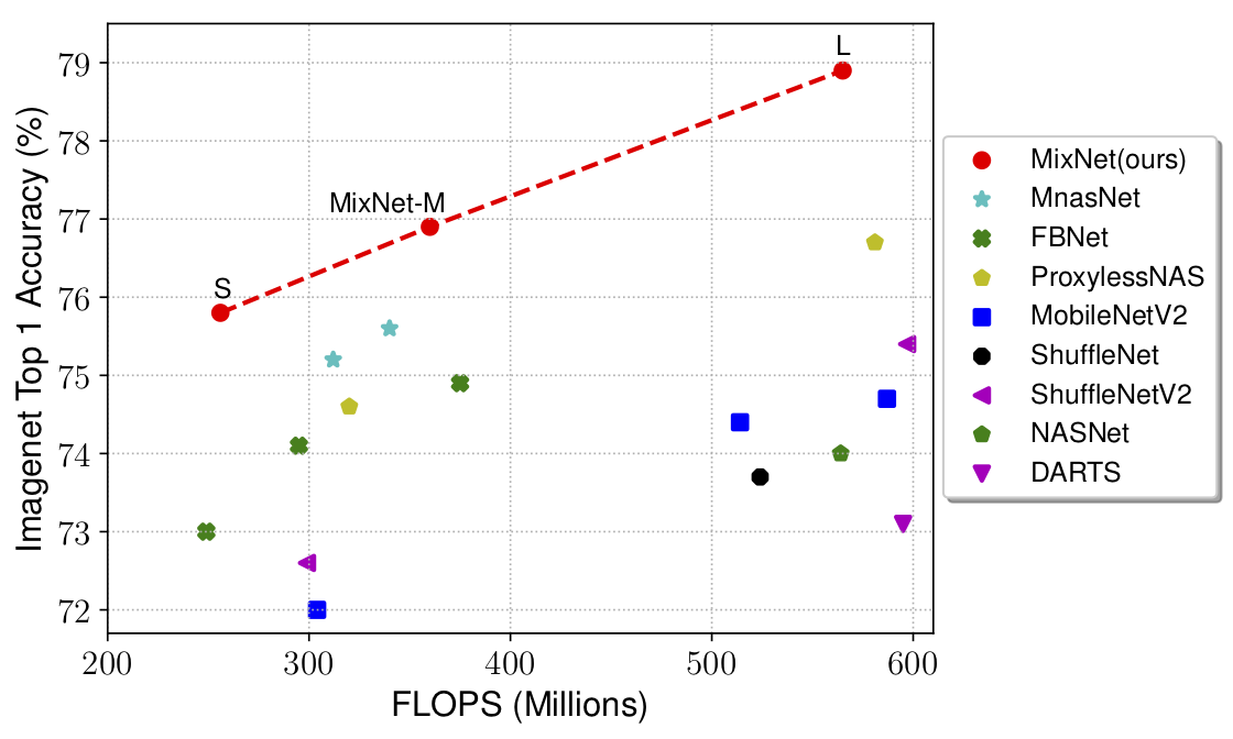
Figure 6-11. Comparison of several mobile-friendly models in the paper “MixNet: Mixed Depthwise Convolution Kernels” by Mingxing Tan and Quoc V. Le
As practitioners, where can we find current state-of-the-art models? PapersWithCode.com/SOTA showcases leaderboards on several AI problems, comparing paper results over time, along with the model code. Of particular interest would be the models with a low number of parameters that achieve high accuracies. For example, EfficientNet gets an amazing Top-1 84.4% accuracy with 66 million parameters, so it could be an ideal candidate for running on servers. Additionally, the ImageNet test metrics are on 1,000 classes, whereas our case might just require classification on a few classes. For those cases, a much smaller model would suffice. Models listed in Keras Application (tf.keras.applications), TensorFlow Hub, and TensorFlow Models usually carry many variations (input image sizes, depth multipliers, quantizations, etc.).
Tip
Shortly after Google AI researchers publish a paper, they release the model used in the paper on the TensorFlow Models repository.
Quantize the Model
“Represent 32-bit weights to 8-bit integer, get 2x faster, 4x smaller models”
Neural networks are driven primarily by matrix–matrix multiplications. The arithmetic involved tends to be rather forgiving in that small deviations in values do not cause a significant swing in output. This makes neural networks fairly robust to noise. After all, we want to be able to recognize an apple in a picture, even in less-than-perfect lighting. When we quantize, we essentially take advantage of this “forgiving” nature of neural networks.
Before we look at the different quantization techniques, let’s first try to build an intuition for it. To illustrate quantized representations with a simple example, we’ll convert 32-bit floating-point weights to INT8 (8-bit integer) using linear quantization. Obviously, FP32 represents 232 values (hence, 4 bytes to store), whereas INT8 represents 28 = 256 values (1 byte). To quantize:
-
Find the minimum and maximum values represented by FP32 weights in the neural network.
-
Divide this range into 256 intervals, each corresponding to an INT8 value.
-
Calculate a scaling factor that converts an INT8 (integer) back to a FP32. For example, if our original range is from 0 to 1, and INT8 numbers are 0 to 255, the scaling factor will be 1/256.
-
Replace FP32 numbers in each interval with the INT8 value. Additionally, store the scaling factor for the inference stage where we convert INT8 values back to FP32 values. This scaling factor only needs to be stored once for the entire group of quantized values.
-
During inference calculations, multiply the INT8 values by the scaling factor to convert it back to a floating-point representation. Figure 6-12 illustrates an example of linear quantization for the interval [0, 1].

Figure 6-12. Quantizing from a 0 to 1 32-bit floating-point range down to an 8-bit integer range for reduced storage space
There are a few different ways to quantize our models, the simplest one being reducing the bit representation of the weights from 32-bit to 16-bit or lower. As might be evident, converting 32-bit to 16-bit means half the memory size is needed to store a model. Similarly, converting to 8-bit would require a quarter of the size. So why not convert it to 1-bit and save 32x the size? Well, although the models are forgiving up to a certain extent, with each reduction, we will notice a drop in accuracy. This reduction in accuracy grows exponentially beyond a certain threshold (especially below 8 bits). To go below and still have a useful working model (like a 1-bit representation), we’d need to follow a special conversion process to convert them to binarized neural networks. XNOR.ai, a deep learning startup, has famously been able to bring this technique to production. The Microsoft Embedded Learning Library (ELL) similarly provides such tools, which have a lot of value for edge devices like the Raspberry Pi.
There are numerous benefits to quantization:
- Improved memory usage
-
By quantizing to 8-bit integer representation (INT8), we typically get a 75% reduction in model size. This makes it more convenient to store and load the model in memory.
- Improved performance
-
Integer operations are faster than floating-point operations. Additionally, the savings in memory usage reduces the likelihood of having to unload the model from RAM during execution, which also has the added benefit of decreased power consumption.
- Portability
-
Edge devices such as Internet of Things devices might not support floating-point arithmetic, so it would be untenable to keep the model as a floating-point in such situations.
Most inference frameworks provide a way to quantize, including Core ML Tools from Apple, TensorRT from NVIDIA (for servers), and TensorFlow Lite, as well as the TensorFlow Model Optimization Toolkit from Google. With TensorFlow Lite, models can be quantized after training during conversion (called post-training quantization). To minimize accuracy losses even further, we can use the TensorFlow Model Optimization Toolkit during training. This process is called quantization-aware training.
It would be useful to measure the benefit provided by quantization. Metrics from the TensorFlow Lite Model optimization benchmarks (shown in Table 6-4) give us a hint, comparing 1) unquantized, 2) post-training quantized, and 3) quantization-aware trained models. The performance was measured on a Google Pixel 2 device.
| Model | MobileNet | MobileNetV2 | InceptionV3 | |
|---|---|---|---|---|
|
Top-1 accuracy |
Original |
0.709 | 0.719 | 0.78 |
|
Post-training quantized |
0.657 | 0.637 | 0.772 | |
|
Quantization-aware training |
0.7 | 0.709 | 0.775 | |
|
Latency (ms) |
Original |
124 | 89 | 1130 |
|
Post-training quantized |
112 | 98 | 845 | |
|
Quantization-aware training |
64 | 54 | 543 | |
|
Size (MB) |
Original |
16.9 | 14 | 95.7 |
|
Optimized |
4.3 | 3.6 | 23.9 | |
So, what do these numbers indicate? After quantization using TensorFlow Lite to INT8, we see roughly a four-times reduction in size, approximately two-times speedup in run time, and less than 1% change in accuracy. Not bad!
More extreme form of quantization, like 1-bit binarized neural networks (like XNOR-Net), claim a whopping 58-times speedup with roughly 32-times smaller size when tested on AlexNet, with a 22% loss in accuracy.
Prune the Model
Pick a number. Multiply it by 0. What do we get? Zero. Multiply your pick again by a small value neighboring 0, like 10–6, and we’ll still get an insignificant value. If we replace such tiny weights (→ 0) in a model with 0 itself, it should have little effect on the model’s predictions. This is called magnitude-based weight pruning, or simply pruning, and is a form of model compression. Logically, putting a weight of 0 between two nodes in a fully connected layer is equivalent to deleting the edge between them. This makes a model with dense connections sparser.
As it happens, a large chunk of the weights in a model are close to 0. Pruning the model will result in many of those weights being set to 0. This happens with little impact to accuracy. Although this does not save any space by itself, it introduces a ton of redundancy that can be exploited when it comes time to save the model to disk in a compressed format such as ZIP. (It is worth noting that compression algorithms thrive on repeating patterns. The more the repetition, the higher the compressibility.) The end result is that our model can often be compressed by four times. Of course, when we finally need to use the model, it would need to be uncompressed before loading in memory for inference.
The TensorFlow team observed the accuracy loss shown in Table 6-5 while pruning the models. As expected, more efficient models like MobileNet observe higher (though still small) accuracy loss when compared with comparatively bigger models like InceptionV3.
| Model | Sparsity | Accuracy loss against original accuracy |
|---|---|---|
| InceptionV3 | 50% | 0.1% |
| InceptionV3 | 75% | 2.5% |
| InceptionV3 | 87.5% | 4.5% |
| MobileNet | 50% | 2% |
Keras provides APIs to prune our model. This process can be done iteratively during training. Train a model normally or pick a pretrained model. Then, periodically prune the model and continue training. Having enough epochs between the periodic prunes allows the model to recover from any damage due to introducing so much sparsity. The amount of sparsity and number of epochs between prunes can be treated as hyperparameters to be tuned.
Another way of implementing this is by using Tencent’s PocketFlow tool, a one-line command that provides several other pruning strategies implemented in recent research papers.
Use Fused Operations
In any serious CNN, the convolutional layer and batch normalization layer frequently appear together. They are kind of the Laurel and Hardy of CNN layers. Fundamentally, they are both linear operations. Basic linear algebra tells us that combining two or more linear operations will also result in a linear operation. By combining convolutional and batch normalization layers, we not only reduce the number of computations, but also decrease the amount of time spent in data transfer, both between main memory and GPU, and main memory and CPU registers/cache. Making them one operation prevents an extra roundtrip. Luckily, for inference purposes, most inference frameworks either automatically do this fusing step or provide model converters (like TensorFlow Lite) to make this optimization while converting the model to the inference format.
Enable GPU Persistence
Loading and initializing the GPU drivers take time. You might have noticed a delay every time a training or inference job was initiated. For frequent, short jobs, the overhead can become relatively expensive quickly. Imagine an image classification program for which the classification takes 10 seconds, 9.9 of which were spent in loading the driver. What we need is for the GPU driver to stay preinitialized in the background, and be ready for whenever our training jobs start. And that’s where the NVIDIA GPU Persistence Daemon comes to the rescue:
$ nvidia-persistenced --user {YOUR_USERNAME}
Our GPUs will use a bit more wattage during idle time, but they will be ready and available the next time a program is launched.
Summary
In this chapter, we explored different avenues for improving the speed and performance of our deep learning pipeline, from storing and reading the data to inference. A slow data pipeline often leads to a GPU starving for data, resulting in idle cycles. With several of the simple optimizations we discussed, our hardware can be put to its maximum efficiency. The handy checklist can serve as a ready reference. Feel free to make a copy for your desk (or your refrigerator). With these learnings, we hope to see your entry among the top performers of the MLPerf benchmark list.