
Appendix A. A Crash Course in Convolutional Neural Networks
In keeping with the word “practical” in the book’s title, we’ve focused heavily on the real-world aspects of deep learning. The goal of this appendix is meant to serve as reference material, rather than a full-fledged exploration into the theoretical aspects of deep learning. To develop a deeper understanding of some of these topics, we recommend perusing the “Further Exploration” for references to other source material.
Machine Learning
-
Machine learning helps learn patterns from data to make predictions on unseen data.
-
There are three kinds of machine learning: supervised learning (learning from labeled data), unsupervised learning (learning from unlabeled data), and reinforcement learning (learning by action and feedback from an environment).
-
Supervised learning tasks include classification (output is one of many categories/classes) and regression (output is a numeric value).
-
There are various supervised machine learning techniques including naive Bayes, SVM, decision trees, k-nearest neighbors, neural networks, and others.
Perceptron
-
A perceptron, as shown in Figure A-1, is the simplest form of a neural network, a single-layered neural network with one neuron.
-
A perceptron calculates a weighted sum of its inputs; that is, it accepts input values, multiplies each with a corresponding weight, adds a bias term, and generates a numeric output.

Figure A-1. An example of a perceptron
-
Because a perceptron is governed by a linear equation, it only has the capacity to model linear or close-to-linear tasks well. For a regression task, the prediction can be represented as a straight line. For a classification task, the prediction can be represented as a straight line separating a plane into two parts.
-
Most practical tasks are nonlinear in nature, and hence a perceptron would fail to model the underlying data well, leading to poor prediction performance.
Activation Functions
-
Activation functions convert linear input into nonlinear output. A sigmoid (Figure A-2) is a type of activation function. The hyperbolic tangent function and ReLU, shown in Figure A-3 are other common activation functions.

Figure A-2. A plot of the sigmoid function
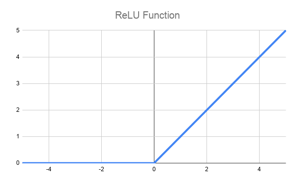
Figure A-3. A plot of the ReLU function
-
For classification, the probability of predicting a category is usually desired. This can be accomplished by a sigmoid function (for binary classification tasks) at the end of the perceptron, which converts values in the range of 0 to 1, and hence is better suited to represent probabilities.
-
Activation functions help replicate the biological concept of the firing of neurons, which, in the simplest case, can be on or off; that is, the inputs activate the neurons. A step function is one form of an activation function where the value is one when the neuron is activated and zero when not. One downside of using a step function is that it loses the magnitude. ReLU, on the other hand, outputs the magnitude of the activation if it activates, and zero otherwise. Due to its simplicity and low computational requirements, it is preferred for nonprobability-based outputs.
Neural Networks
-
Combining a perceptron with a nonlinear activation function improves its predictive ability. Combining several perceptions with nonlinear activation functions improves it even further.
-
A neural network, as seen in Figure A-4, consists of multiple layers, each containing multiple perceptrons. Layers are connected in a sequence, passing the output of the previous layer as the input to the subsequent layer. This data transfer is represented as connections, with each neuron connected to every neuron in the previous and subsequent layers (hence the layers are aptly named fully connected layers). Each of these connections has a multiplying factor associated with it, also known as a weight.

Figure A-4. An example of a multilayer neural network
-
Each neuron stores the associated weights and bias, and has an optional nonlinear activation function at the end of it.
-
Since information flows in one direction, without any cycles, this network structure is also called a feedforward neural network or multilayer feedforward network.
-
The layers between the input(s) and output(s), hidden from the end-user, are appropriately known as hidden layers.
-
Neural networks have a powerful ability to model patterns in data (i.e., represent the underlying relationship between data and associated labels). The Universal Approximation Theorem states that a neural network with a single hidden layer can represent any continuous function within a specific range, acting as a universal approximator. So technically, a single-layer network could model any problem in existence. The major caveat is that it might be infeasible in practice due to the sheer number of neurons required to model many problems. The alternative approach is to have multiple layers with a fewer number of neurons per layer, which works well in practice.
-
The output of a single hidden layer is the result of a nonlinear function applied over a linear combination of its inputs. The output of a second hidden layer is the result of a nonlinear function applied over a linear combination of inputs, which itself are nonlinear functions applied over a linear combination of their inputs. Each layer further builds upon the predictive power of the previous layer. Thus, the higher the number of layers, the better the representative ability of the neural network to model real-world nonlinear problems. This makes the network deep, and hence such networks with many hidden layers are also called deep neural networks.
Backpropagation
-
Training a network involves modifying the weights and biases of the network iteratively until the network starts to make predictions with minimal error.
-
Backpropagation helps train neural networks. It involves making a prediction, measuring how far-off the prediction is from the ground truth, and propagating the error back into the network so that the weights can be updated in order to reduce the magnitude of the error in subsequent iterations. This process is repeated until the error of the network no longer reduces.
-
Neural networks are usually initialized with random weights.
-
The performance of a model is measured with loss functions. For regression tasks (with numeric predictions), mean squared error (MSE) is a commonly used loss function. Due to the squaring of the magnitude of the error, using MSE helps favor more small errors than a few large errors. For classification tasks (with category predictions), the cross-entropy loss is commonly used. While accuracy is used more as a human-understandable metric of performance, cross-entropy loss is used for training a network, since it’s more nuanced.
Shortcoming of Neural Networks
-
A layer of a neural network with
nneurons andiinputs requiresn x iweights and computations since each neuron is connected to its inputs. An image usually has a lot of pixels as inputs. For an image with widthw, heighth, andcchannels,w x h x c x ncomputations would be required. For a standard smartphone camera’s image (usually 4032 x 3024 pixels in 3 channels of red, green, and blue), if the first hidden layer has 128 neurons, over 4 billion weights and computations would result, making neural networks impractical to use for most computer-vision tasks. We want to ideally convert an image into a much smaller workable representation that can then be classified by a neural network. -
Pixels in an image usually are related to other pixels in their vicinity. Capturing this relationship can give a better understanding of the image’s content. But while feeding a neural network, the relationship between these pixels is lost because the image is flattened out into a 1D array.
Desired Properties of an Image Classifier
-
It captures relationships between different parts of an image.
-
It is resilient to differences in position, size, angle of an object present in an image, and other factors such as noise. That is, an image classifier should be invariant to geometric transformations (often referred to using terms such as translation invariance, rotational invariance, positional invariance, shift-invariance, scale invariance, etc.).
-
A CNN satisfies many of these desired properties in practice (some by its design, others with data augmentation).
Convolution
-
A convolutional filter is a matrix that slides across an image (row by row, left to right), and multiplies with that section of adjoining pixels to produce an output. Such filters are famously used in Photoshop to blur, sharpen, brighten, darken an image, etc.
-
Convolutional filters can, among other things, be used to detect vertical, horizontal, and diagonal edges. That is, when edges are present, they generate higher numbers as output, and lower output values otherwise. Alternatively stated, they “filter” out the input unless it contains an edge.
-
Historically, convolutional filters were hand-engineered to perform a task. In the context of neural networks, these convolutional filters can be used as building blocks whose parameters (matrix weights) can be deduced automatically via a training pipeline.
-
A convolutional filter activates every time it spots the input pattern it has been trained for. Since it traverses over an entire image, the filter is capable of locating the pattern at any position in the image. As a result, the convolutional filters contribute to making the classifier position invariant.
Pooling
-
A pooling operation reduces the spatial size of the input. It looks at smaller portions of an input and performs an aggregation operation reducing the output to a single number. Typically aggregation operations include finding the maximum or average of all values, also commonly known as max pooling and average pooling, respectively. For example, a
2 x 2max pooling operation will replace each2 x 2submatrix of the input (without overlap) with a single value in the output. Similar to convolution, pooling traverses the entire input matrix, aggregating multiple blocks of values into single values. If the input matrix were of size2N x 2N, the resulting output would be of sizeN x N. -
In the aforementioned example, the output would be the same regardless of where in the
2 x 2matrix the maximum occurred. -
Max pooling is more commonly used than average pooling because it acts as a noise suppressor. Because it only takes the maximum value in each operation, it ignores the lower values, which are typically characteristics of noise.
Structure of a CNN
-
At a high level, a CNN (shown in Figure A-5) consists of two parts—a featurizer followed by a classifier. The featurizer reduces the input image to a workable size of features (i.e., a smaller representation of the image) upon which the classifier then acts.
-
A CNN’s featurizer is a repeating structure of convolutional, activation, and pooling layers. The input passes through this repeating structure in a sequence one layer at a time.

Figure A-5. A high-level overview of a convolutional network
-
The transformed input is finally passed into classification layers, which are really just neural networks. In this context, the classification neural network is typically known as a fully connected layer.
-
Much like in neural networks, the nonlinearity provided by activation functions help the CNN learn complex features. ReLU is the most commonly used activation function.
-
Empirically, earlier layers (i.e., those closer to the input layers) detect simple features such as curves and edges. If a matching feature is detected, the layer gets activated and passes on the signal to subsequent layers. Eventual layers combine these signals to detect more complex features such as a human eye, human nose, or human ears. Ultimately, these signals might add up to detect the entire object such as a human face.
-
CNNs are trained using backpropagation just like multilayer perceptron networks.
-
Unlike traditional machine learning, this makes feature selection automated. Additionally, the reduction of the input into smaller features makes the process more computationally efficient. Both of these are big selling points of deep learning.
Further Exploration
The topics we cover in this book should be self-sufficient, but if you do choose to develop a deeper appreciation for the underlying fundamentals, we highly recommend checking out some of the following material:
- https://www.deeplearning.ai
-
This set of deep learning courses from Andrew Ng covers the foundations for a wide range of topics, encompassing theoretical knowledge and deep insights behind each concept.
- https://course.fast.ai
-
This course by Jeremy Howard and Rachel Thomas has a more hands-on approach to deep learning using PyTorch as the primary deep learning framework. The fast.ai library used in this course has helped many students run models with state-of-the-art performance using just a few lines of code.
- Hands-On Machine Learning with Scikit-Learn, Keras, and TensorFlow, 2nd Edition
-
This book by Aurélien Géron covers machine learning and delves into topics such as support vector machines, decision trees, random forests, etc., then bridges into deep learning topics such as convolutional and recurrent neural networks. It explains both theory as well as some hands-on examples of these techniques.