
Chapter 17. Building an Autonomous Car in Under an Hour: Reinforcement Learning with AWS DeepRacer
If you follow technology news, you probably have seen a resurgence in debates about when computers are going to take over the world. Although that’s a fun thought exercise, what’s triggered the resurgence in these debates? A large part of the credit can be attributed to the news of computers beating humans at decision-making tasks—winning in chess, achieving high scores in video games like Atari (2013), beating humans in a complex game of Go (2016), and, finally, beating human teams at Defence of the Ancients (Dota) 2 in 2017. The most astonishing thing about these successes is that the “bots” learned the games by playing against one another and reinforcing the strategies that they found to bring them success.
If we think more broadly on this concept, it’s no different than how humans teach their pets. To train a dog, every good behavior is reinforced by rewarding the dog with a treat and lots of hugs, and every undesired behavior is discouraged by asserting “bad doggie.” This concept of reinforcing good behaviors and discouraging bad ones essentially forms the crux of reinforcement learning.
Computer games, or games in general, require a sequence of decisions to be made, so traditional supervised methods aren’t well suited, because they often focus on making a single decision (e.g., is this an image of a cat or a dog?). The inside joke in the reinforcement learning community is that we just play video games all day (spoiler alert: It’s true!). At present, reinforcement learning is being applied across industries to optimize stock trading, manage heating and cooling in large buildings and datacenters, perform real-time bidding of advertisements, optimize video-streaming quality, and even optimize chemical reactions in a lab. Given these examples of production systems, we would strongly advocate using reinforcement learning for sequential decision making and optimization problems. In this chapter, we focus on learning this paradigm of machine learning and applying it to a real-world problem: building a one-eighteenth-scale, self-driving autonomous car in less than an hour.
A Brief Introduction to Reinforcement Learning
Similar to deep learning, reinforcement learning has seen a renaissance in the past few years ever since previously held human video game records were broken. Reinforcement learning theory had its heyday in the 1990s, but didn’t break in to large-scale production systems due to computational requirements and difficulty in training these systems. Traditionally reinforcement learning has been considered compute heavy; in contrast, neural networks are data heavy. But advancements in deep neural networks have also benefited reinforcement learning. Neural networks are now being used to represent the reinforcement learning model, thus giving birth to deep reinforcement learning. In this chapter, we use the term reinforcement learning and deep reinforcement learning interchangeably, but in almost all cases if not stated otherwise, when we refer to reinforcement learning, we are talking about deep reinforcement learning.
Despite recent advancements, the landscape for reinforcement learning has not been developer friendly. Interfaces for training deep learning models have progressively become simpler, but this hasn’t quite caught up in the reinforcement learning community. Another challenging aspect for reinforcement learning has been the significant computational requirements and time to model convergence (it has completed learning)—it literally takes days, if not weeks, to create a converged model. Now, assuming that we had the patience, knowledge of neural networks, and the monetary bandwidth, educational resources regarding reinforcement learning are few and far between. Most of the resources are targeted to advanced data scientists, and sometimes out of reach for developers. That one-eighteenth-scale autonomous car we referenced earlier? That’s AWS’ DeepRacer (Figure 17-1). One of the biggest motivations behind AWS DeepRacer was to make reinforcement learning accessible to developers. It is powered by Amazon SageMaker reinforcement learning, which is a general-purpose reinforcement learning platform. And, let’s get real: who doesn’t like self-driving cars?

Figure 17-1. The AWS DeepRacer one-eighteenth-scale autonomous car
Why Learn Reinforcement Learning with an Autonomous Car?
In recent years, self-driving technology has seen significant investments and success. DIY self-driving and radio-controlled (RC) car-racing communities have since become popular. This unparalleled enthusiasm in developers building scaled autonomous cars with real hardware, testing in real-world scenarios has compelled us to use a “vehicle,” literally, to educate developers on reinforcement learning. Although there existed other algorithms to build self-driving cars, like traditional computer vision or supervised learning (behavioral cloning), we believe reinforcement learning has an edge over these.
Table 17-1 summarizes some of the popular self-driving kits available for developers, and the technologies that enable them. One of the key benefits of reinforcement learning is that models can be trained exclusively in a simulator. But reinforcement learning systems come with their own set of challenges, the biggest of them being the simulation-to-real (sim2real) problem. There’s always a challenge of deploying models trained completely in simulation in to real-world environments. DeepRacer tackles this with some simple, yet effective solutions that we discuss later in the chapter. Within the first six months following the launch of DeepRacer in November 2018, close to 9,000 developers trained their models in the simulator and successfully tested them on a real-world track.
| Hardware | Assembly | Technology | Cost | ||
|---|---|---|---|---|---|
| AWS DeepRacer | Intel Atom with 100 GFLOPS GPU | Preassembled | Reinforcement learning | $399 |
 |
| OpenMV | OpenMV H7 | DIY (two hours) | Traditional computer vision | $90 |
 |
| Duckietown | Raspberry Pi | Preassembled | Reinforcement learning, behavioral cloning | $279–$350 |
 |
| DonkeyCar | Raspberry Pi | DIY (two to three hours) | Behavioral closing | $250 |
 |
| NVIDIA JetRacer | Jetson Nano | DIY (three to five hours) | Supervised learning | ~$400 |
 |
Practical Deep Reinforcement Learning with DeepRacer
Now for the most exciting part of this chapter: building our first reinforcement learning-based autonomous racing model. Before we embark on the journey, let’s build a quick cheat sheet of terms that will help you to become familiar with important reinforcement learning terminology:
- Goal
-
Finishing a lap around the track without going off track.
- Input
-
In a human driven car, the human visualizes the environment and uses driving knowledge to make decisions and navigate the road. DeepRacer is also a vision-driven system and so we use a single camera image as our input into the system. Specifically, we use a grayscale 120x160 image as the input.
- Output (Actions)
-
In the real world, we drive the car by using the throttle (gas), brake, and steering wheel. DeepRacer, which is built on top of a RC car, has two control signals: the throttle and the steering, both of which are controlled by traditional pulse-width modulation (PWM) signals. Mapping driving to PWM signals can be nonintuitive, so we discretize the driving actions that the car can take. Remember those old-school car-racing games we played on the computer? The simplest of those used the arrow keys—left, right, and up—to drive the car. Similarly, we can define a fixed set of actions that the car can take, but with more fine-grained control over throttle and steering. Our reinforcement learning model, after it’s trained, will make decisions on which action to take such that it can navigate the track successfully. We’ll have the flexibility to define these actions as we create the model.
Note
A servo in an RC hobby car is generally controlled by a PWM signal, which is a series of pulses of varying width. The position in which the servo needs to end up is achieved by sending a particular width of the pulse signal. The parameters for the pulses are min pulse width, max pulse width, and repetition rate.
- Agent
-
The system that learns and makes decisions. In our case, it’s the car that’s learning to navigate the environment (the track).
- Environment
-
Where the agent learns by interacting with actions. In DeepRacer, the environment contains a track that defines where the agent can go and be in. The agent explores the environment to collect data to train the underlying deep reinforcement learning neural network.
- State (s)
-
The representation of where the agent is in an environment. It’s a point-in-time snapshot of the agent. For DeepRacer, we use an image as the state.
- Actions (a)
-
Set of decisions that the agent can make.
- Step
-
Discrete transition from one state to the next.
- Episode
-
This refers to an attempt by the car to achieve its goal; that is, complete a lap on the track. Thus, an episode is a sequence of steps, or experience. Different episodes can have different lengths.
- Reward (r)
-
The value for the action that the agent took given an input state.
- Policy (π)
-
Decision-making strategy or function; a mapping from state to actions.
- Value function (V)
-
The mapping of state to values, in which value represents the expected reward for an action given the state.
- Replay or experience buffer
-
Temporary storage buffer that stores the experience, which is a tuple of (s,a,r,s
'), where “s” stands for an observation (or state) captured by the camera, “a” for an action taken by the vehicle, “r” for the expected reward incurred by the said action, and “s'” for the new observation (or new state) after the action is taken. - Reward function
-
Any reinforcement learning system needs a guide, something that tells the model as it learns what’s a good or a bad action given the situation. The reward function acts as this guide, which evaluates the actions taken by the car and gives it a reward (scalar value) that indicates the desirability of that action for the situation. For example, on a left turn, taking a “left turn” action would be considered optimal (e.g., reward = 1; on a 0–1 scale), but taking a “right turn” action would be bad (reward = 0). The reinforcement learning system eventually collects this guidance based on the reward function and trains the model. This is the most critical piece in training the car and the part that we’ll focus on.
Finally, when we put together the system, the schematic flow looks as follows:
Input (120x160 grayscale Image) → (reinforcement learning Model) →
Output (left, right, straight)
In AWS DeepRacer, the reward function is an important part of the model building process. We must provide it when training our AWS DeepRacer model.
In an episode, the agent interacts with the track to learn the optimal set of actions it needs to take to maximize the expected cumulative reward. But a single episode doesn’t produce enough data for us to train the agent. So, we end up collecting many episodes’ worth of data. Periodically, at the end of every nth episode, we kick off a training process to produce an iteration of the reinforcement learning model. We run many iterations to produce the best model we can. This process is explained in detail in the next section. After the training, the agent executes autonomous driving by running inference on the model to take an optimal action given an image input. The evaluation of the model can be done in either the simulated environment with a virtual agent or a real-world environment with a physical AWS DeepRacer car.
It’s finally time to create our first model. Because the input into the car is fixed, which is a single image from the camera, we need to focus only on the output (actions) and the reward function. We can follow the steps below to begin training the model.
Building Our First Reinforcement Learning
To do this exercise, you will need an AWS account. Log into the AWS Console using your account credentials, as shown in Figure 17-2.

Figure 17-2. The AWS login console
First, let’s make sure we are in the North Virginia region, given that the service is available only in that region, and then navigate to the DeepRacer console page: https://console.aws.amazon.com/deepracer/home?region=us-east-1#getStarted.
After you select “Reinforcement learning,” the model page opens. This page shows a list of all the models that have been created and the status of each model. To create a model, start the process here.

Figure 17-3. Workflow for training the AWS DeepRacer model
Step 1: Create Model
We are going to create a model that can be used by the AWS DeepRacer car to autonomously drive (take actions) around a race track. We need to select the specific race track, provide the actions that our model can choose from, provide a reward function that will be used to incentivize our desired driving behavior, and configure the hyperparameters used during training.

Figure 17-4. Creating a model on the AWS DeepRacer console
Step 2: Configure Training
In this step, we select our training environment, configure action space, write our reward function, and adjust other training related settings before kicking off our training job.
Configure the simulation environment
Training our reinforcement learning model takes place on a simulated race track, and we can choose the track to train our model. We’ll use AWS RoboMaker, a cloud service that makes building robotic applications easy, to spin up the simulation environment.
When training a model, we pick the track most similar to the final track we intend to race on. As of July 2019, AWS DeepRacer provides seven tracks that we can train on. While configuring such a complementary environment isn’t required and doesn’t guarantee a good model, it will maximize the odds that our model will perform best on the race track. Furthermore, if we train on a straight track, it’s unlikely that our model would have learned how to turn. Just like in the case of supervised learning in which it’s unlikely that the model will learn something that’s not part of the training data, in reinforcement learning, the agent is unlikely to learn anything out of scope from the training environment. For our first exercise, select the re:Invent 2018 track, as shown in Figure 17-5.
To train a reinforcement learning model, we must choose a learning algorithm. Currently, the AWS DeepRacer console supports only the proximal policy optimization (PPO) algorithm. The team eventually will support more algorithms, but PPO was chosen for faster training times and superior convergence properties. Training a reinforcement learning model is an iterative process. First, it’s a challenge to define a reward function to cover all important behaviors of an agent in an environment at once. Second, hyperparameters are often tuned to ensure satisfactory training performance. Both require experimentation. A prudent approach is to start with a simple reward function, which will be our approach in this chapter, and then progressively enhance it. AWS DeepRacer facilitates this iterative process by enabling us to clone a trained model, in which we could enhance the reward function to handle previous ignored variables or we can systematically adjust hyperparameters until the result converges. The easiest way to detect this convergence is look at the logs and see whether the car is going past the finish line; in other words, whether progress is 100%. Alternatively, we could visually observe the car’s behavior and confirm that it goes past the finish line.

Figure 17-5. Track selection on the AWS DeepRacer console
Configure the action space
Next, we configure the action space that our model will select both during and after training. An action (output) is a combination of speed and steering angle. Currently in AWS DeepRacer, we use a discrete action space (a fixed set of actions) as opposed to a continuous action space (turn x degrees with y speed, where x and y take real values). This is because it’s easier to map to values on the physical car, which we dive into later in the “Racing the AWS DeepRacer Car” To build this discrete action space, we specify the maximum speed, the speed levels, the maximum steering angle, and the steering levels, as depicted in Figure 17-6.

Figure 17-6. Defining the action space on the AWS DeepRacer console
Following are the configuration parameters for the action space:
- Maximum steering angle
-
This is the maximum angle in degrees that the front wheels of the car can turn to the left and to the right. There is a limit as to how far the wheels can turn, and so the maximum turning angle is 30 degrees.
- Steering angle granularity
-
Refers to the number of steering intervals between the maximum steering angle on either side. Thus, if our maximum steering angle is 30 degrees, +30 degrees is to the left and –30 degrees is to the right. With a steering granularity of 5, the following steering angles, as shown in Figure 17-6, from left to right, will be in the action space: 30 degrees, 15 degrees, 0 degrees, –15 degrees, and –30 degrees. Steering angles are always symmetrical around 0 degrees.
- Maximum speed
-
Refers to the maximum speed the car will drive in the simulator as measured in meters per second (m/s).
- Speed levels
-
Refers to the number of speed levels from the maximum speed (including) to zero (excluding). So, if our maximum speed is 3 m/s and our speed granularity is 3, our action space will contain speed settings of 1 m/s, 2 m/s, and 3 m/s. Simply put, 3 m/s divided by 3 = 1 m/s, so go from 0 m/s to 3 m/s in increments of 1 m/s. 0 m/s is not included in the action space.
Based on the previous example the final action space will include 15 discrete actions (three speeds x five steering angles), which should be listed in the AWS DeepRacer service. Feel free to tinker with other options, just remember that larger action spaces might take a bit longer to train.
Tip
Based on our experience, here are some tips on how to configure the action space:
-
Our experiments have shown that models with a faster maximum speed take longer to converge than those with a slower maximum speed. In some cases (reward function and track dependent), it can take longer than 12 hours for a 5 m/s model to converge.
-
Our model will not perform an action that is not in the action space. Similarly, if the model is trained on a track that never required the use of this action—for example, turning won’t be incentivized on a straight track—the model won’t know how to use this action, because it won’t be incentivized to turn. As you begin thinking about building a robust model, make sure that you keep the action space and training track in mind.
-
Specifying a fast speed or a wide steering angle is great, but we still need to think about our reward function and whether it makes sense to drive full speed into a turn, or exhibit zigzag behavior on a straight section of the track.
-
We also need to keep physics in mind. If we try to train a model at faster than 5 m/s, we might see our car spin out on corners, which will probably increase the time to convergence of our model.
Configure reward function
As we explained earlier, the reward function evaluates the quality of an action’s outcome given the situation, and rewards the action accordingly. In practice the reward is calculated during training after each action is taken, and forms a key part of the experience used to train the model. We then store the tuple (state, action, next state, reward) in a memory buffer. We can build the reward function logic using a number of variables that are exposed by the simulator. These variables represent measurements of the car, such as steering angle and speed; the car in relation to the racetrack, such as (x, y) coordinates; and the racetrack, such as waypoints (milestone markers on the track). We can use these measurements to build our reward function logic in Python 3 syntax.
All of the parameters are available as a dictionary to the reward function. Their keys, data types, and descriptions are documented in Figure 17-7, and some of the more nuanced ones are further illustrated in Figure 17-8.

Figure 17-7. Reward function parameters (a more in-depth review of these parameters is available in the documentation)

Figure 17-8. Visual explanation of some of the reward function parameters
To build our first model, let’s pick an example reward function and train our model. Let’s use the default template, shown in Figure 17-9, in which the car tries to follow the center dashed lines. The intuition behind this reward function is to take the safest navigation path around the track because being in the center keeps the car farthest from being off track. The reward function does the following: creates three tiers around the track, using the three markers, and then proceeds to reward the car more for driving in the second tier as opposed to the center or the last tier. Also note the differences in the size of the reward. We provide a reward of 1 for staying in the narrow center tier, 0.5 for staying in the second (off-center) tier, and 0.1 for staying in the last tier. If we decrease the reward for the center tier, or increase the reward for the second tier, we are essentially incentivizing the car to use a larger portion of the track surface. Remember that time you did your driving test? The examiner probably did the same and cut off points as you got closer to the curb or the lane makers. This could come in handy, especially when there are sharp corners.

Figure 17-9. An example reward function
Here’s the code that sets this up:
defreward_function(params):'''Example of rewarding the agent to follow center line'''# Read input parameterstrack_width=params['track_width']distance_from_center=params['distance_from_center']# Calculate 3 markers that are at varying distances away from the center linemarker_1=0.1*track_widthmarker_2=0.25*track_widthmarker_3=0.5*track_width# Give higher reward if the car is closer to center line and vice versaifdistance_from_center<=marker_1:reward=1.0elifdistance_from_center<=marker_2:reward=0.5elifdistance_from_center<=marker_3:reward=0.1else:reward=1e-3# likely crashed/ close to off trackreturnfloat(reward)
Because this is the first training run, let’s focus on understanding the process of creating and evaluating a basic model, and then focus on optimizing it. In this case, we skip the algorithm settings and hyperparameter sections and use the defaults.
Note
FAQ: Should the rewards be in a certain range, and also can I give negative rewards?
There are no real constraints on what we can reward and not reward, but as a good practice it’s easier to understand rewards when they are in a 0–1 or 0–100 scale. What’s more important is that our reward scale gives relative rewards for the actions appropriately. For example, on a right turn, we should reward the right action with high reward, a left action with close to 0 reward, perhaps a straight action with an in-between reward or higher than the left action because it might not be a completely bad action to take.
Configure stop conditions
This is the last section before we begin training. Here we specify the maximum time our model will train for. This is provided as a convenient mechanism for us to terminate our training given that we are billed for the amount of training time.
Specify 60 minutes and then select “Start training.” If there is an error, we will be taken to the error location. After we start training, it can take up to six minutes to spin up the services (such as Amazon SageMaker, AWS Robomaker, AWS Lambda, AWS Step Function) needed to start training. Remember, we can always stop training early if we determine that the model has converged (as explained in the next section) by clicking the “stop” button.
Step 3: Model Training
After our model has begun training, we can select it from the listed models on the DeepRacer console. We can then see quantitatively how the training is progressing by looking at the total reward over time graph and also qualitatively from a first-person view from the car in the simulator (see Figure 17-10).
At first, our car will not be able to drive on a straight road, but as it learns better driving behavior, we should see its performance improving and the reward graph increasing. Furthermore, when our car drives off of the track it will be reset on the track. We might observe that the reward graph is spiky.
Note
FAQ: Why is the reward graph spiky?
The agent starts with high exploration, and gradually begins to exploit the trained model. Because the agent always takes random actions for a fraction of its decisions, there might be occasions for which it totally makes the wrong decision and ends up going off track. This is typically high at the beginning of training, but eventually the spikiness should reduce as the model begins to learn.
Logs are always a good source of more granular information regarding our model’s training. Later in the chapter, we examine how we can use the logs programmatically to gain a deeper understanding of our model training. In the meantime, we can look at the log files for both Amazon SageMaker and AWS RoboMaker. The logs are output to Amazon CloudWatch. To see the logs, hover your mouse over the reward graph and select the three dots that appear below the refresh button. Then, select “View logs.” Because the model training will take an hour, this might be a good time to skip to the next section and learn a bit more about reinforcement learning.

Figure 17-10. Training graph and simulation video stream on the AWS DeepRacer console
Step 4: Evaluating the Performance of the Model
In reinforcement learning, the best way to gauge the ability of the model is to run it such that it only exploits—that is, it doesn’t take random actions. In our case, first test it on a track similar to the one it’s trained on to see whether it can replicate the trained behavior. Next, try it on a different track to test generalizability. After our model training is complete, we can commence model evaluation. From our model details page, where we observed training, select “Start evaluation.” We can now select the track on which we want to evaluate the performance of our model and also the number of laps. Select the “re:Invent 2018” track and 5 laps and then select Start. When it’s done, we should see a similar page as that shown in Figure 17-11, which summarizes the results of our model’s attempts to go around the track and complete the lap.

Figure 17-11. Model evaluation page on the AWS DeepRacer console
Great job! We have successfully built our first reinforcement learning–enabled autonomous car.
Note
FAQ: When I run evaluation, I see only 100% completion rates sometimes?
As the model runs inference and navigates around the track in the simulator, due to the fidelity of the simulator, the car can end up in slightly different positions for the same action—in other words, a 15 degree left turn action might result in only 14.9 degrees. Practically, we observe only very small deviations in the simulator, but these small deviations can add up over time. A well-trained model is able to recover from close-to-off-track positions, but an undertrained model is likely to not recover from close calls.
Now that our model has been successfully evaluated, we move on to improving it and learn to achieve better lap times. But before that, it’s necessary for you to understand more about the theory behind reinforcement learning and dig deeper into the learning process.
Reinforcement Learning in Action
Let’s take a closer look at reinforcement learning in action. Here, we discuss some theory, the inner workings, and lots of practical insights related to our autonomous car project.
How Does a Reinforcement Learning System Learn?
First, we must understand explore versus exploit. Similar to how a child learns, a reinforcement learning system learns from exploring and finding out what’s good and bad. In the case of the child, the parent guides or informs the child of its mistakes, qualifies the decisions made as good or bad, or to what degree they were good or bad. The child memorizes the decisions it took for given situations and tries to replay, or exploit, those decisions at opportune moments. In essence, the child is trying to maximize the parent’s approval or cheer. Early in a child’s life, it’s more attentive to the suggestions from its parents, thus creating opportunities to learn. And later in life, as adults who seldom listen to their parents, exploit the concepts they have learned to make decisions.
As shown in Figure 17-12, at every timestep “t,” the DeepRacer car (agent) receives its current observation, the state (St), and on that basis the car selects an action (At). As a result of the action the agent took, it gets a reward Rt+1 and moves to state St+1, and this process continues throughout the episode.

Figure 17-12. Reinforcement learning theory basics in a nutshell
In the context of DeepRacer, the agent explores by taking random actions, and the reward function, which essentially acts just like the parent, tells the car whether the actions it took for the given state were good or not. Usually, “goodness” of the action for a given state is expressed as a number, with higher numbers meaning it’s close to optimal and lower meaning it’s not. The system records all of this information for every step, specifically: current state, action taken, reward for the action, and next state (s,a,r,s'), in what we call the experience replay buffer, which is essentially a temporary memory buffer. The entire idea here being that the car can learn from what decisions were good and other decisions that were bad. The key point is that we start with a high degree of exploration, and slowly increase exploitation.
In the DeepRacer simulator, we sample the input image state at 15 frames per second. At each step or image frame captured, the car transitions from one state to another. Each image represents the state the car is in, and eventually after the reinforcement learning model is trained, it will look to exploit by inferring which action to take. To make decisions, we could either take random actions or use our model for a recommendation. As the model trains, the training process balances the exploration and exploitation. To begin, we explore more, given that our model is unlikely to be good, but as it learns through experience, we shift more toward exploitation by giving the model more control. Figure 17-13 depicts this flow. This transition could be a linear decay, an exponential decay, or any similar strategy that’s usually tuned based on the degree of learning we hypothesize. Typically, an exponential decay is used in practical reinforcement learning training.

Figure 17-13. The DeepRacer training flow
After an action is taken by a random choice or the model prediction, the car transitions to a new state. Using the reward function, the reward is computed and assigned to the outcome. This process will continue, for each state, until we get to a terminal state; that is, the car goes off track or completes a lap, at which point the car will be reset and then repeated. A step is a transition from one state to another, and at each step a (state, action, new state, reward) tuple is recorded. The collection of steps from the reset point until the terminal state is called an episode.
To illustrate an episode, let’s look at the example of a miniature race track in Figure 17-14, where the reward function incentivizes following the centerline because it’s the shortest and quickest path from start to finish. This episode consists of four steps: at step 1 and 2 the car follows the center line, and then it turns left 45 degrees at step 3, and continues in that direction only to finally crash at step 4.

Figure 17-14. Illustration of an agent exploring during an episode
We can think of these episodes as experience, or training data for our model. Periodically, the reinforcement learning system takes a random subset of these recordings from the memory buffer and trains a DNN (our deep reinforcement learning model) to produce a model that can best navigate the environment based on our reward function “guide”; in other words, get maximum cumulative rewards. As time progresses or with more episodes, we see a model that becomes better over time. Of course, the supercritical caveat being that the reward function is well defined and directing the agent toward the goal. If our reward function is bad, our model will not learn the correct behavior.
Let’s take a slight diversion to understand a bad reward function. As we were initially designing the system, the car had freedom to go in any direction (left, right, forward, back). Our simplest reward function didn’t distinguish between directions, and in the end the model learned the best way to accumulate awards by just rocking backward and forward. This was then overcome by incentivizing the car to go forward. Luckily for developers now, the DeepRacer team made it simpler by allowing the car to move only in the forward direction, so we don’t even need to think of such behavior.
Now back to reinforcement learning. How do we know if the model is getting better? Let’s return to the concepts of explore and exploit. Remember that we begin with high exploration, low exploitation, and gradually increase the rate of exploitation. This means that at any point in the training process, for a certain percentage of time the reinforcement learning system will explore; that is, take random actions. As the experience buffer grows, for any given state, it stores all kinds of decisions (actions) including the ones that resulted in the highest reward to the lowest reward. The model essentially uses this information to learn and predict the best action to take for the given state. Suppose that the model initially took an action “go straight” for state S and received a reward of 0.5, but the next time it arrived in state S, it took action “go right” and received a reward of 1. If the memory buffer had several samples of the reward as “1” for the same state S for action “go right,” the model eventually learns “go right” is the optimal action for that state. Over time, the model will explore less and exploit more, and this percentage allocation is changed either linearly or exponentially to allow for the best learning.
The key here is that if the model is taking optimal actions, the system learns to keep selecting those actions; if it isn’t selecting the best action, the system continues to try to learn the best action for a given state. Practically speaking, there can exist many paths to get to the goal, but for the mini racetrack example in Figure 17-13, the fastest path is going to be right down the middle of the track, as practically speaking any turns would slow down the car. During training, in early episodes as the model begins to learn, we observe that it might end up at the finish line (goal) but might not be taking the optimal path, as illustrated in Figure 17-15 (left) where the car zigzags, thus taking more time to get to the finish line and earning cumulative rewards of only 9. But because the system still continues to explore for a fraction of the time, the agent gives itself opportunities to find better paths. As more experience is built, the agent learns to find an optimal path and converge to an optimal policy to reach the goal with total cumulative rewards of 18, as illustrated in Figure 17-15 (right).

Figure 17-15. Illustration of different paths to the goal
Quantitatively speaking, for each episode, you should see a trend of increasing rewards. If the model is making those optimal decisions, the car must be on track and navigating the course, resulting in accumulating rewards. However, you might see even after high reward episodes the graph dipping, which can happen in early episodes because the car might still have a high degree of exploration, as mentioned earlier.
Reinforcement Learning Theory
Now that we understand how a reinforcement learning system learns and works, especially in the context of AWS DeepRacer, let’s look at some formal definitions and general reinforcement learning theory. This background will be handy when we solve other problems using reinforcement learning.
The Markov decision process
Markov decision process (MDP) is a discrete stochastic state-transition process framework that is used for modeling decision making in a control process. The markov property defines that each state is solely dependent on the previous state. This is a convenient property because it means that to make a state transition, all of the necessary information must be available in the current state. Theoretical results in reinforcement learning rely on the problem being formulated as an MDP, hence it’s important to understand how to model a problem as an MDP to be solved using reinforcement learning.
Model free versus model based
Model, in this context, refers to the learned representation of the environment. This is useful because we can potentially learn the dynamics in the environment and train our agent using the model rather than having to use the real environment every time. However, in reality, learning the environment isn’t easy, and it’s often easier to have a representation of the real world in simulation and then jointly learn both perception and dynamics as part of the agent navigation rather than one after the other in a sequence. In this chapter, we focus only on model-free reinforcement learning.
Value based
For every action taken by the agent, there’s a corresponding reward assigned by the reward function. For any given state-action pair, it’s helpful to know its value (reward). If such a function were to exist, we could compute the maximum reward that can be achieved in any state and simply select the corresponding action to navigate the environment. For example, in a game of 3x3 tic-tac-toe, there are a finite number of game situations, so we could build a lookup table to give us the best move given the situation. But in a game of chess, given the size of the board and complexity of the game, such a lookup table would be computationally expensive to build and memory storage would be large. Thus, in a complex environment it’s difficult to tabulate state-action value pairs or define a function that can map state-action pairs to values. So, instead we try to use a neural network by parameterizing the value function and using a neural network to approximate the value for every action given a state observation. An example of a value-based algorithm is Deep Q-Learning.
Policy based
A policy is a set of rules that the agent learns to navigate the environment. Simply put the policy function tells the agent which action is the best action to take from its current state. Policy-based reinforcement learning algorithms like REINFORCE and Policy Gradients find the optimal policy without the need to map values to states. In reinforcement learning, we parameterize the policy. In other words, we allow a neural network to learn what the optimal policy function is.
Policy based or value based—why not both?
There’s always been a debate about whether to use policy-based or value-based reinforcement learning. Newer architectures try to learn both the value function and policy function together rather than keeping one fixed. This approach in reinforcement learning is called actor critic.
You can associate the actor with the policy and the critic with the value function. The actor is responsible for taking actions, and the critic is responsible for estimating the “goodness,” or the value of those actions. The actor maps states to actions, and the critic maps state-action pairs to values. In the actor-critic paradigm, the two networks (actor and critic) are trained separately using gradient ascent to update the weights of our deep neural network. (Remember that our goal is to maximize cumulative rewards; thus, we need to find global maxima.) As the episodes roll by, the actor becomes better at taking actions that lead to higher reward states, and the critic also becomes better at estimating the values of those actions. The signal for both the actor and critic to learn comes purely from the reward function.
The value for a given state-action pair is called Q value, denoted by Q(s,a). We can decompose the Q value into two parts: the estimated value and a quantitative measure of the factor by which the action is better than others. This measure is called the Advantage function. We can view Advantage as the difference between the actual reward for a given state-action pair and the expected reward at that state. The higher the difference, the farther we are from selecting an optimal action.
Given that estimating the value of the state could end up being a difficult problem, we can focus on learning the advantage function. This allows us to evaluate the action not only based on how good it is, but also based on how much better it could be. This allows us to converge to an optimal policy much easier than other simpler policy gradient-based methods because, generally, policy networks have high variance.
Delayed rewards and discount factor (γ)
Rewards are given for every state transition based on the action taken. But the impact of these rewards might be nonlinear. For certain problems the immediate rewards might be more important, and in some cases the future rewards more important. As an example, if we were to build a stock-trading algorithm, the future rewards might have higher uncertainty; thus, we would need to discount appropriately. The discount factor (γ) is a multiplication factor between [0,1], where closer to zero indicates rewards in the immediate future are more important. With a high value that’s closer to 1, the agent will focus on taking actions that maximize future rewards.
Reinforcement Learning Algorithm in AWS DeepRacer
First, let’s look at one of the simplest examples of a policy optimization reinforcement learning algorithm: vanilla policy gradient.

Figure 17-16. Training process for the vanilla policy gradient algorithm
We can think of a deep reinforcement learning model as consisting of two parts: the input embedder and policy network. The input embedder will extract features from the image input and pass it to the policy network, which makes decisions; for instance, predict which action is the best for the given input state. Given that our input is an image, we use convolution layers (CNNs) to extract features. Because the policy is something we want to learn, we parameterize our policy function, the simplest of which can be learned with a fully connected layer. The input CNN layers take in an image and then the policy network uses the image features as input and outputs an action. Thus, mapping state to action. As the model trains, we become better at mapping the input space and extracting relevant features and also optimizing the policy to get the best action for each state. Our goal here is to collect maximum cumulative rewards. To achieve that, our model weights are updated such to maximize the cumulative future reward, and in doing so, we give a higher probability to the action that leads to the higher cumulative future reward. In training neural networks previously, we used stochastic gradient descent or its variation; when training an reinforcement learning system, we seek to maximize the cumulative reward; so, instead of minimization, we look to maximize. So, we use gradient ascent to move the weights in the direction of the steepest reward signal.
DeepRacer uses an advanced variation of policy optimization, called Proximal Policy Optimization (PPO), summarized in Figure 17-17.
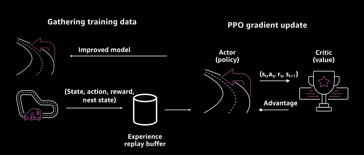
Figure 17-17. Training using the PPO algorithm
On the left side of Figure 17-17, we have our simulator using the latest policy (model) to get new experience (s,a,r,s'). The experience is fed into an experience replay buffer that feeds our PPO algorithm after we have a set number of episodes.
On the right side of Figure 17-17, we update our model using PPO. Although PPO is a policy optimization method, it uses the advantage actor-critic method, which we described earlier. We compute the PPO gradient and shift policy in the direction where we get the highest rewards. Blindly taking large steps in this direction can cause too much variability in training; if we take small steps training can take forever. PPO improves the stability of the policy (actor) by limiting how much the policy can update at each training step. This is done by using a clipped surrogate objective function, which prevents the policy from being updated too much, thus solving large variance, a common issue with policy optimization methods. Typically, for PPO, we keep the ratio of new and old policy at [0.8, 1.2]. The critic tells the actor how good the action taken was, and how the actor should adjust its network. After the policy is updated the new model is sent to the simulator to get more experience.
Deep Reinforcement Learning Summary with DeepRacer as an Example
To solve any problem with reinforcement learning, we need to work through the following steps:
-
Define the goal.
-
Select the input state.
-
Define the action space.
-
Construct the reward function.
-
Define the DNN architecture.
-
Pick the reinforcement learning optimization algorithm (DQN, PPO, etc.).
The fundamental manner in which a reinforcement learning model trains doesn’t change if we are building a self-driving car or building a robotic arm to grasp objects. This is a huge benefit of the paradigm because it allows us to focus on a much higher level of abstraction. To solve a problem using reinforcement learning, the main task at hand is to define our problem as an MDP, followed by defining the input state and set of actions that the agent can take in a given environment, and the reward function. Practically speaking, the reward function can be one of the most difficult parts to define, and often is the most important as this is what influences the policy that our agent learns. After all the environment-dependent factors are defined, we can then focus on what the deep neural network architecture should be to map the input to actions, followed by picking the reinforcement learning algorithm (value-based, policy-based, actor-critic-based) to learn. After we pick the algorithm, we can focus on the high level knobs to control what the algorithm does. When we drive a car, we tend to focus on controls, and the understanding of the internal combustion engine doesn’t influence too much the way we drive. Similarly, as long as we understand the knobs that each algorithm exposes, we can train a reinforcement learning model.
It’s time to bring this home. Let’s formulate the DeepRacer racing problem:
-
Goal: To finish a lap by going around the track in the least amount of time
-
Input: Grayscale 120x160 image
-
Actions: Discrete actions with combined speed and steering angle values
-
Rewards: Reward the car for being on the track, incentivize going faster, and prevent from doing a lot of corrections or zigzag behavior
-
DNN architecture: Three-layer CNN + fully connected layer (Input → CNN → CNN → CNN → FC → Output)
-
Optimization algorithm: PPO
Step 5: Improving Reinforcement Learning Models
We can now look to improve our models and also get insights into our model training. First, we focus on training improvements in the console. We have at our disposal the ability to change the reinforcement learning algorithm settings and neural network hyperparameters.
Algorithm settings
This section specifies the hyperparameters that will be used by the reinforcement learning algorithm during training. Hyperparameters are used to improve training performance.
Hyperparameters for the neural network
Table 17-2 presents the hyperparameters that are available to tune the neural network. Even though the default values have experimentally proven to be good, practically speaking the developer should focus on the batch size, number of epochs, and the learning rate as they were found to be the most influential in producing high-quality models; that is, getting the best out of our reward function.
| Parameter | Description | Tips |
|---|---|---|
| Batch size | The number recent of vehicle experiences sampled at random from an experience buffer and used for updating the underlying deep learning neural network weights. If we have 5,120 experiences in the buffer, and specify a batch size of 512, then ignoring random sampling, we will get 10 batches of experience. Each batch will be used, in turn, to update our neural network weights during training. | Use a larger batch size to promote more stable and smooth updates to the neural network weights, but be aware of the possibility that the training may be slower. |
| Number of epochs | An epoch represents one pass through all batches, where the neural network weights are updated after each batch is processed, before proceeding to the next batch. Ten epochs implies we update the neural network weights, using all batches one at a time, but repeat this process 10 times. | Use a larger number of epochs to promote more stable updates, but expect slower training. When the batch size is small, we can use a smaller number of epochs. |
| Learning rate | The learning rate controls how big the updates to the neural network weights are. Simply put, when we need to change the weights of our policy to get to the maximum cumulative reward, how much should we shift our policy. | A larger learning rate will lead to faster training, but it may struggle to converge. Smaller learning rates lead to stable convergence, but can take a long time to train. |
| Exploration | This refers to the method used to determine the trade-off between exploration and exploitation. In other words, what method should we use to determine when we should stop exploring (randomly choosing actions) and when should we exploit the experience we have built up. | Since we will be using a discrete action space, we should always select “CategoricalParameters.” |
| Entropy | A degree of uncertainty, or randomness, added to the probability distribution of the action space. This helps promote the selection of random actions to explore the state/action space more broadly. | |
| Discount factor | A factor that specifies how much the future rewards contribute to the expected cumulative reward. The larger the discount factor, the farther out the model looks to determine the expected cumulative reward and the slower the training. With a discount factor of 0.9, the vehicle includes rewards from an order of 10 future steps to make a move. With a discount factor of 0.999, the vehicle considers rewards from an order of 1,000 future steps to make a move. | The recommended discount factor values are 0.99, 0.999, and 0.9999. |
| Loss type | The loss type specifies the type of the objective function (cost function) used to update the network weights. The Huber and mean squared error loss types behave similarly for small updates. But as the updates become larger, the Huber loss takes smaller increments compared to the mean squared error loss. | When we have convergence problems, use the Huber loss type. When convergence is good and we want to train faster, use the mean squared error loss type. |
| Number of episodes between each training | This parameter controls how much experience the car should obtain between each model training iteration. For more complex problems that have more local maxima, a larger experience buffer is necessary to provide more uncorrelated data points. In this case, training will be slower but more stable. | The recommended values are 10, 20, and 40. |
Insights into model training
After the model is trained, at a macro level the rewards over time graph, like the one in Figure 17-10, gives us an idea of how the training progressed and the point at which the model begins to converge. But it doesn’t give us an indication of the converged policy, insights into how our reward function behaved, or areas where the speed of the car could be improved. To help gain more insights, we developed a Jupyter Notebook that analyzes the training logs, and provides suggestions. In this section, we look at some of the more useful visualization tools that can be used to gain insight into our model’s training.
The log file records every step that the car takes. At each step it records the x,y location of the car, yaw (rotation), the steering angle, throttle, the progress from the start line, action taken, reward, the closest waypoint, and so on.
Heatmap visualization
For complex reward functions, we might want to understand reward distribution on the track; that is, where did the reward function give rewards to the car on the track, and its magnitude. To visualize this, we can generate a heatmap, as shown in Figure 17-18. Given that the reward function we used gave the maximum rewards closest to the center of the track, we see that region to be bright and a tiny band on either side of the centerline beyond it to be red, indicating fewer rewards. Finally, the rest of the track is dark, indicating no rewards or rewards close to 0 were given when the car was in those locations. We can follow the code to generate our own heatmap and investigate our reward distribution.

Figure 17-18. Heatmap visualization for the example centerline reward function
Improving the speed of our model
After we run an evaluation, we get the result with lap times. At this point, we might be curious as to the path taken by the car or where it failed, or perhaps the points where it slowed down. To understand all of these, we can use the code in this notebook to plot a race heatmap. In the example that follows, we can observe the path that the car took to navigate around the track and also visualize the speeds at which it passes through at various points on the track. This gives us insight into parts that we can optimize. One quick look at Figure 17-19 (left) indicates that the car didn’t really go fast at the straight part of the track; this provides us with an opportunity. We could incentivize the model by giving more rewards to go faster at this part of the track.

Figure 17-19. Speed heatmap of an evaluation run; (left) evaluation lap with the basic example reward function, (right) faster lap with modified reward function
In Figure 17-19 (left), it seems like the car has a small zigzag pattern at times, so one improvement here could be that we penalize the car when it turns too much. In the code example that follows, we multiply the reward by a factor of 0.8, if the car is steering beyond a threshold. We also incentivize the car to go faster by giving 20% more reward if the car goes at 2 m/s or more. When trained with this new reward function, we can see that the car does go faster than the previous reward function. Figure 17-19 (right) shows more stability; the car follows the centerline almost to perfection and finishes the lap roughly two seconds faster than our first attempt. This is just a glimpse in to improving the model. We can continue to iterate on our models and clock better lap times using these tools. All of the suggestions are incorporated in to the reward function example shown here:
defreward_function(params):'''Example of penalize steering, which helps mitigate zigzag behaviors andspeed incentive'''# Read input parametersdistance_from_center=params['distance_from_center']track_width=params['track_width']steering=abs(params['steering_angle'])# Only need absolute steering anglespeed=params['speed']# in meter/sec# Calculate 3 markers that are at varying distances away from the center linemarker_1=0.1*track_widthmarker_2=0.25*track_widthmarker_3=0.5*track_width# Give higher reward if the agent is closer to the center line and vice versaifdistance_from_center<=marker_1:reward=1elifdistance_from_center<=marker_2:reward=0.5elifdistance_from_center<=marker_3:reward=0.1else:reward=1e-3# likely crashed/ close to off track# Steering penalty threshold, change the number based on your action spacesettingABS_STEERING_THRESHOLD=15# Penalize reward if the agent is steering too muchifsteering>ABS_STEERING_THRESHOLD:reward*=0.8# Incentivize going fasterifspeed>=2:reward*=1.2
Racing the AWS DeepRacer Car
It’s time to bring what we’ve learned so far from the virtual to the physical world and race a real autonomous car. Toy sized, of course!
If you own an AWS DeepRacer car, follow the instructions provided to test your model on a physical car. For those interested in buying the car, AWS DeepRacer is available for purchase on Amazon.
Building the Track
Now that we have a trained model, we can evaluate this model on a real track and with a physical AWS DeepRacer car. First, let’s build a makeshift track at home to race our model. For simplicity, we’ll build only part of a racetrack, but instructions on how to build an entire track are provided here.
To build a track, you need the following materials:
- For track borders:
-
We can create a track with tape that is about two-inches wide and white or off-white color against the dark-colored track surface. In the virtual environment, the thickness of the track markers is set to be two inches. For a dark surface, use a white or off-white tape. For example, 1.88-inch width, pearl white duct tape or 1.88-inch (less sticky) masking tape.
- For track surface:
-
We can create a track on a dark-colored hard floor such as hardwood, carpet, concrete, or asphalt felt. The latter mimics the real-world road surface with minimal reflection.
AWS DeepRacer Single-Turn Track Template
This basic track template consists of two straight track segments connected by a curved track segment, as illustrated in Figure 17-20. Models trained with this track should make our AWS DeepRacer vehicle drive in a straight line or make turns in one direction. The angular dimensions for the turns specified are suggestive; we can use approximate measurements when laying down the track.

Figure 17-20. The test track layout
Running the Model on AWS DeepRacer
To start the AWS DeepRacer vehicle on autonomous driving, we must upload at least one AWS DeepRacer model to our AWS DeepRacer vehicle.
To upload a model, pick our trained model from the AWS DeepRacer console and then download the model artifacts from its Amazon S3 storage to a (local or network) drive that can be accessed from the computer. There’s an easy download model button provided on the model page.
To upload a trained model to the vehicle, do the following:
-
From the device console’s main navigation pane, choose Models, as shown in Figure 17-21.

Figure 17-21. The Model upload menu on the AWS DeepRacer car web console
-
On the Models page, above the Models list, choose Upload.
-
From the file picker, navigate to the drive or share where you downloaded the model artifacts and choose the model for upload.
-
When the model is uploaded successfully, it will be added to the Models list and can be loaded into the vehicle’s inference engine.
Driving the AWS DeepRacer Vehicle Autonomously
To start autonomous driving, place the vehicle on a physical track and do the following:
-
Follow the instructions to sign in to the vehicle’s device console, and then do the following for autonomous driving:
-
On the “Control vehicle” page, in the Controls section, choose “Autonomous driving,” as shown in Figure 17-22.

Figure 17-22. Driving mode selection menu on the AWS DeepRacer car web console
-
-
On the “Select a model” drop-down list (Figure 17-23), choose an uploaded model, and then choose “Load model.” This will start loading the model into the inference engine. The process takes about 10 seconds to complete.
-
Adjust the “Maximum speed” setting of the vehicle to be a percentage of the maximum speed used in training the model. (Certain factors such as surface friction of the real track can reduce the maximum speed of the vehicle from the maximum speed used in the training. You’ll need to experiment to find the optimal setting.)

Figure 17-23. Model selection menu on AWS DeepRacer car web console
-
Choose “Start vehicle” to set the vehicle to drive autonomously.
-
Watch the vehicle drive on the physical track or the streaming video player on the device console.
-
To stop the vehicle, choose “Stop vehicle.”
Sim2Real transfer
Simulators can be more convenient than the real world to train on. Certain scenarios can be easily created in a simulator; for example, a car colliding with a person or another car—we wouldn’t want to do this in the real world :). However, the simulator in most cases will not have the visual fidelity we do in the real world. Also, it might not be able to capture the physics of the real world. These factors can affect modeling the environment in the simulator, and as a result, even with great success in simulation, when the agent runs in the real world, we can experience failures. Here are some of the common approaches to handle the limitations of the simulator:
- System identification
-
Build a mathematical model of the real environment and calibrate the physical system to be as realistic as possible.
- Domain adaptation
-
Map the simulation domain to the real environment, or vice versa, using techniques such as regularization, GANs, or transfer learning.
- Domain randomization
-
Create a variety of simulation environments with randomized properties and train a model on data from all these environments.
In the context of DeepRacer, the simulation fidelity is an approximate representation of the real world, and the physics engine could use some improvements to adequately model all the possible physics of the car. But the beauty of deep reinforcement learning is that we don’t need everything to be perfect. To mitigate large perceptual changes affecting the car, we do two major things: a) instead of using an RGB image, we grayscale the image to make the perceptual differences between the simulator and the real world narrower, and b) we intentionally use a shallow feature embedder; for instance, we use only a few CNN layers; this helps the network not learn the simulation environment entirely. Instead it forces the network to learn only the important features. For example, on the race track the car learns to focus on navigating using the white track extremity markers. Take a look at Figure 17-24, which uses a technique called GradCAM to generate a heatmap of the most influential parts of the image to understand where the car is looking for navigation.

Figure 17-24. GradCAM heatmaps for AWS DeepRacer navigation
Further Exploration
To continue with the adventure, you can become involved in various virtual and physical racing leagues. Following are a few options to explore.
DeepRacer League
AWS DeepRacer has a physical league at AWS summits and monthly virtual leagues. To race in the current virtual track and win prizes, visit the league page: https://console.aws.amazon.com/deepracer/home?region=us-east-1#leaderboards.
Advanced AWS DeepRacer
We understand that some advanced developers might want more control over the simulation environment and also have the ability to define different neural network architectures. To enable this experience, we provide a Jupyter Notebook–based setup with which you can provision the components needed to train your custom AWS DeepRacer models.
AI Driving Olympics
At NeurIPS 2018, the AI Driving Olympics (AI-DO) was launched with a focus on AI for self-driving cars. During the first edition, this global competition featured lane-following and fleet-management challenges on the Duckietown platform (Figure 17-25). This platform has two components, Duckiebots (miniature autonomous taxis), and Duckietowns (miniature city environments featuring roads, signs). Duckiebots have one job—to transport the citizens of Duckietown (the duckies). Onboard with a tiny camera and running the computations on Raspberry Pi, Duckiebots come with easy-to-use software, helping everyone from high schoolers to university researchers to get their code running relatively quickly. Since the first edition of the AI-DO, this competition has expanded to other top AI academic conferences and now includes challenges featuring both Duckietown and DeepRacer platforms.

Figure 17-25. Duckietown at the AI Driving Olympics
DIY Robocars
The DIY Robocars Meetup, initially started in Oakland (California), now has expanded to more than 50 meetup groups around the world. These are fun and engaging communities to try and work with other enthusiasts in the self-driving and autonomous robocar space. Many of them run monthly races and are great venues to physically race your robocar.
Roborace
It’s time to channel our inner Michael Schumacher. Motorsports is typically considered a competition of horsepower, and now Roborace is turning it into a competition of intelligence. Roborace organizes competitions between all-electric, self-driving race cars, like the sleek-looking Robocar designed by Daniel Simon (known for futuristic designs like the Tron Legacy Light Cycle), shown in Figure 17-26. We are not talking about miniature-scaled cars anymore. These are full-sized, 1,350 kg, 4.8 meters, capable of reaching 200 mph (320 kph). The best part? We don’t need intricate hardware knowledge to race them.
The real stars here are AI developers. Each team gets an identical car, so that the winning edge is focused on the autonomous AI software written by the competitors. Output of onboard sensors such as cameras, radar, lidar, sonar, and ultrasonic sensors is available. For high-throughput computations, the cars are also loaded with the powerful NVIDIA DRIVE platform capable of processing several teraflops per second. All we need to build is the algorithm to let the car stay on track, avoid getting into an accident, and of course, get ahead as fast as possible.
To get started, Roborace provides a race simulation environment where precise virtual models of real cars are available. Along comes virtual qualification rounds, where the winners get to participate in real races including at Formula E circuits. By 2019, the top racing teams have already closed the gap to within 5–10% of the best human performances in races. Soon developers will be standing on top of the podium, after beating professional drivers. Ultimately, competitions like these lead to innovations and hopefully the learnings can be translated back to the autonomous car industry, making them safer, more reliable, and performant at the same time.

Figure 17-26. Robocar from Roborace designed by Daniel Simon (image courtesy of Roborace)
Summary
In the previous chapter, we looked at how to train a model for an autonomous vehicle by manually driving inside the simulator. In this chapter, we explored concepts related to reinforcement learning and learned how to formulate the ultimate problem on everyone’s mind: how to get an autonomous car to learn how to drive. We used the magic of reinforcement learning to remove the human from the loop, teaching the car to drive in a simulator on its own. But why limit it to the virtual world? We brought the learnings into the physical world and raced a real car. And all it took was an hour!
Deep reinforcement learning is a relatively new field but an exciting one to explore further. Some of the recent extensions to reinforcement learning are opening up new problem domains where its application can bring about large-scale automation. For example, hierarchical reinforcement learning allows us to model fine-grained decision making. Meta-RL allows us to model generalized decision making across environments. These frameworks are getting us closer to mimicking human-like behavior. It’s no surprise that a lot of machine learning researchers believe reinforcement learning has the potential to get us closer to artificial general intelligence and open up avenues that were previously considered science fiction.