Appendix B

Survival Distributions

B.1 Introduction

The survival distributions we discuss here are all available as functions in R. The most basic survival distribution is the Exponential distribution, not because it is useful as is in demographic applications (it isn’t), but because it is a reference distribution, a special case of other distributions, and a building block in many useful models.

The piecewise constant hazards, Gamma, and the Weibull distributions are all generalizations of the exponential.

B.2 Relevant Distributions in R

In R, there are several families of distributions available. The ones that are relevant in survival analysis are characterized by having positive support. For each family of distributions, four functions are available; a density function (name prefix d), a cumulative distribution function (name prefix p), a quantile function (name prefix q), and a random number generator (name prefix r). In the package eha, the two functions with prefix ‘h’ and ‘H’ are added for some distributions. For instance, for the Weibull distribution there are hweibull and Hweibull, where the first is the hazard function and the second is the cumulative hazards function.

In Section B.2.1, The Exponential distribution, we show exactly what these functions are and how to use them. It should be noted that in base R, there are no survival functions, hazard functions, or cumulative hazards functions. Some are available in the package eha and others. However, they can easily be derived from the given p- and d- functions, as shown in Section B.2.1.

B.2.1 The Exponential Distribution

The exponential distribution is characterized by having a constant hazard rate λ. It has density function

$\begin{array}{ll}f\left(t;\lambda \right)=\lambda e^{-\lambda x},\hfill & \lambda 0,t>0,\hfill \end{array}$

and survival function

$\begin{array}{ll}S\left(t;\lambda \right)=e^{-\lambda x},\hfill & \lambda >0,t>0.\hfill \end{array}$

The mean is 1/λ (which, unfortunately, also is the scale parameter), and the variance is 1/λ2. The exponential distribution is represented in R by the functions pexp, dexp, qexp, and rexp, in order the cumulative distribution function, the density function, the quantile function (which is the inverse to the cumulative distribution function), and the random number generator function.

In Figure B.1, the relevant functions are plotted for an exponential distribution with λ = 1 (the default value). It is created as follows.

> require(eha)

> x <- seq(0, 4, length = 1000)

> oldpar <- par(mfrow = c(2, 2))

> plot(x, dexp(x), type = “l”,

   main = “Density”, ylab = “”)

> plot(x, pexp(x, lower.tail = FALSE), type = “l”,

   main = “Survival”, ylab = “”)

> plot(x, hweibull(x, shape = 1), type = “l”,

   main = “Hazard”, ylab = “”)

> plot(x, Hweibull(x, shape = 1), type = “l”,

   main = “Cumulative hazards”, ylab = “”)

> par(oldpar)

Note that there are no functions hexp or Hexp, maybe because they are too simple, see Figure B.1. The fact that the exponential distribution is special case of the Weibull distribution (shape = 1) is utilized. The exponential distribution is characterized by the fact that it lacks memory. In other words, items whose life lengths follow an exponential distribution do not age; no matter how old they are, if they are alive they are as good as new. This concept is not useful when it comes to human lives, but the life lengths of electronic components are often modeled by the exponential distribution in reliability theory.

B.2.2 The Piecewise Constant Hazard Distribution

If the exponential distribution is not useful in describing human lives, it may be so for short segments of life. At least it will be a good approximation if the segment is short enough.

This is the idea behind the piecewise constant hazards distribution, called pch in eha. Its definition involves a partition of time (age) axis, and one positive constant (the hazard level) corresponding to each interval. Note that the last interval will be open, with infinite length; only a finite number of cut points are allowed. The definition of the hazard function h becomes, with the cuts denoted t = (t1, < · · · < tn) and the levels denoted h = (h1, ..., hn + 1):

$\begin{array}{ll}h\left(t;\mathrm{t},\mathrm{h}\right)=\{\begin{array}{ll}{h}_1\hfill & t\le t_1,\hfill \\ h_i\hfill & t_{i-1}<t\le t_i,i=2,...,n,\hfill \\ h_{n+1}\hfill & t_n<t.\hfill \end{array}\hfill & (\mathrm{B}.1)\hfill \end{array}$

In this definition, the number of levels must be exactly one more than the number of cut points. The relevant functions are shown in Figure B.2, created as follows:

> cuts <- c(1, 2, 3)

> levels <- c(1, 2, 1, 2)

> par(mfrow = c(2, 2))

> plot(x, dpch(x, cuts = cuts, levels = levels),

   type = “l”, main = “Density”)

> plot(x, ppch(x, cuts = cuts, levels = levels, lower.tail = FALSE),

   type = “l”, main = “Survival”)

> plot(x, hpch(x, cuts = cuts, levels = levels),

   type = “l”, main = “Hazard”, ylab = “”, ylim = c(0, 2.2))

> plot(x, Hpch(x, cuts = cuts, levels = levels),

   type = “l”, main = “Cumulative hazards”)

Note that, despite the fact that the hazard function is not continuous, the other functions are. They are not differentiable at the cut points, though.

The piecewise constant distribution is very flexible. It can be made arbitrarily close to any continuous distribution by increasing the number of cut points and choose the levels appropriately. Parametric proportional hazards modeling with the pch distribution is a serious competitor to the Cox regression model, especially with large data sets.

B.2.3 The Weibull Distribution

The Weibull distribution is a very popular parametric model for survival data, described in detail by Waloddi Weibull (Weibull 1951), known earlier. It is one of the so-called extreme-value distributions, and as such very useful in reliability theory. It is becoming popular in demographic applications, but in mortality studies it is wise to avoid it for old age mortality (the hazard grows too slow) and mortality in ages 0–15 years of age (U-shaped hazards, which the Weibull model doesn’t allow).

The hazard function of a Weibull distribution is defined by

$\begin{array}{ll}h\left(t;\left(p,\lambda \right)\right)=\frac{p}{\lambda }{\left(\frac{t}{\lambda }\right)}^{p-1},\hfill & t,p,\lambda >0.\hfill \end{array}$

where p is a shape parameter and λ is a scale parameter. When p = 1, this reduces to h(t; (1, λ) = 1/λ, which is the exponential distribution with rate 1/λ. Compare to the definition of the exponential distribution and note that there λ is the rate and here it is a scale parameter, which is the inverted value of the rate.

B.2.3.1 Graphical Test of the Weibull Distribution

As mentioned above, the Weibull distribution has a long history in reliability theory. Early on simple graphical tests were constructed for judging if a real data set could be adequately described by the Weibull distribution. The so-called Weibull paper was invented. Starting with the definition of the cumulative hazards function H,

$H\left(t;\left(p,\lambda \right)\right)={\left(\frac{t}{\lambda }\right)}^p,$

by taking logarithms of both sides, we get

$\ln H\left(t;\left(p,\lambda \right)\right)=p\ln \left(t\right)-p\ln \left(\lambda \right)$

with x = ln t and y = ln H(t), this is a straight line. So by plotting the Nelson–Aalen estimator of the cumulative hazards function against log time, it is possible to graphically check the Weibull and exponential assumptions.

Example 32 Male mortality and the Weibull distribution

Is it reasonable to assume that the survival data in the data set mort can be modeled by the Weibull distribution? We construct the Weibull plot as follows.

> data(mort)

> with(mort, plot(Surv(enter, exit, event), fn = “loglog”))

The result is shown in Figure B.3

Except for the early disturbance, linearity is not too far away (remember that the log transform magnifies the picture close to zero; exp(-1.5) is only 0.22 years). Is the slope close to 1? Probably not, the different scales on the axis makes it hard to judge exactly. We can estimate the parameters with the phreg function.

> fit <- phreg(Surv(enter, exit, event) ˜ 1, data = mort)

> fit

Call:

phreg(formula = Surv(enter, exit, event) ˜ 1, data = mort)

Covariate  W.mean  Coef Exp(Coef) se(Coef) Wald p

log(scale)    3.785 44.015 0.066 0.000

log(shape)    0.332 1.393 0.058 0.000

Events    276

Total timeatrisk  17038

Max. log. likelihood -1399.3

The estimate of the shape parameter is 1.393, and it is significantly different from 1 (p = 0.000), so we can firmly reject the hypothesis that data come from an exponential distribution.

B.2.4 The Lognormal Distribution

The lognormal distribution is connected to the normal distribution through the exponential function: If X is normally distributed, then Y = exp(X) is lognormally distributed. Conversely, if Y is lognormally distributed, then X = log(Y) is normally distributed.

The lognormal distribution has the interesting property that the hazard function is first increasing, then decreasing, in contrast to the Weibull distribution which only allows for monotone (increasing or decreasing) hazard functions.

The R functions are named (dpqrhH)lnorm.

B.2.5 The Loglogistic Distribution

The loglogistic distribution is very close to the lognormal, but have heavier tail to the right. Its advantage over the lognormal is that the hazard function has closed form. It is given by

$\begin{array}{ll}h\left(t;\left(p,\lambda \right)\right)=\frac{\frac{p}{\lambda }{\left(\frac{t}{\lambda }\right)}^{p-1}}{1+{\left(\frac{t}{\lambda }\right)}^p},\hfill & t,p,\lambda >0.\hfill \end{array}$

With shape p = 2 and scale λ = 1, its appearance is shown in Figure B.4. It is produced by the code

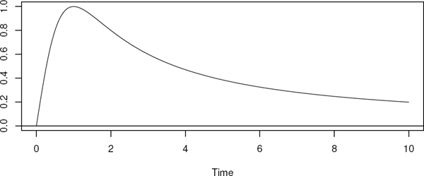
> x <- seq(0, 10, length = 1000)

> plot(x, hllogis(x, shape = 2, scale = 1),

   type = “l”, ylab = ““, xlab = ”Time”)

> abline(h = 0)

The R functions are named (dpqrhH)llogis.

B.2.6 The Gompertz Distribution

The Gompertz distribution is useful for modeling old age mortality. The hazard function is exponentially increasing.

$\begin{array}{ll}h\left(t;\left(p,\lambda \right)\right)=p\exp \left(\frac{t}{\lambda }\right),\hfill & t,p,\lambda >0.\hfill \end{array}$

It was suggested by Gompertz (1825).

The R functions are named (dpqrhH)gamma.

B.2.7 The Gompertz–Makeham Distribution

The Gompertz distribution was generalized by (Makeham 1860). The generalization consists of adding a positive constant to the Gompertz hazard function,

$\begin{array}{ll}h\left(t;\left(\alpha ,p,\lambda \right)\right)=\alpha +p\exp \left(\frac{t}{\lambda }\right),\hfill & t,\alpha ,p,\lambda >0.\hfill \end{array}$

It is more difficult to work with than the other distributions described here. It is not one of the possible choices in the function phreg in eha.

The R functions are named (dpqrhH)makeham.

B.2.8 The Gamma Distribution

The Gamma distribution is another generalization of the exponential distribution. It is popular in modeling shared frailty, see Hougaard (2000). It is not one of the possible distributions for the functions phreg and survreg, and it is not considered further.

The R functions are named (dpqr)gamma.

B.3 Parametric Proportional Hazards and Accelerated Failure Time Models

B.3.1 Introduction

There is a need for software for analyzing parametric proportional hazards (PH) and accelerated failure time (AFT) data, which are right or interval censored and left truncated. The package eha gives one solution to this problem with a specific class of families of survival distributions, but at the time of this writing, interval censoring is not implemented.

The implementation in eha starts with the class of scale/shape families of distributions, to be explained later. The idea is that each family of distributions is generated by shape-scale transformations from any given survival distribution, see Section B.3.3.

B.3.2 The Proportional Hazards Model

We define proportional hazards models in terms of an expansion of a given survival function S0,

$\begin{array}{ll}{s}_{\mathit{\theta }}\left(t;Z\right)={\left\{S_0\left(g\left(t,\mathit{\theta }\right)\right)\right\}}^{\exp \left(\mathbf{z}\beta \right)},\hfill & (\mathrm{B}.2)\hfill \end{array}$

where θ is a parameter vector used in modeling the baseline distribution, β is the vector of regression parameters, and g is a positive function, which helps defining a parametric family of baseline survival functions through

$\begin{array}{llll}S\left(t;\mathit{\theta }\right)=S_0\left(g\left(t,\mathit{\theta }\right)\right),\hfill & t>0,\hfill & \mathit{\theta }\in \Theta .\hfill & (\mathrm{B}.3)\hfill \end{array}$

With f0 and h0 defined as the density and hazard functions corresponding to S0, respectively, the density function corresponding to S is

$\begin{array}{l}f\left(t;\mathit{\theta }\right)=-\frac{\partial }{\partial t}S\left(t,\mathit{\theta }\right)\\ =-\frac{\partial }{\partial t}{S}_0\left(g\left(t,\mathit{\theta }\right)\right)\\ =g_t\left(t,\mathit{\theta }\right)f_0\left(g\left(t,\mathit{\theta }\right)\right),\end{array}$

where

$g_t\left(t,\mathit{\theta }\right)=\frac{\partial }{\partial t}g\left(t,\mathit{\theta }\right).$

Correspondingly, the hazard function is

$\begin{array}{ll}\begin{array}{l}h\left(t;\mathit{\theta }\right)=\frac{f\left(t;\mathit{\theta }\right)}{S\left(t;\mathit{\theta }\right)}\\ =g_t\left(t,\mathit{\theta }\right)h_0\left(g\left(t,\mathit{\theta }\right)\right).\end{array}\hfill & (B.4)\hfill \end{array}$

So, the proportional hazards model is

$\begin{array}{ll}\begin{array}{l}{\lambda }_{\mathit{\theta }}\left(t;\mathbf{z}\right)=h\left(t;\mathit{\theta }\right)\exp \left(\mathbf{z}\beta \right)\\ =g_t\left(t,\mathit{\theta }\right)h_0\left(g\left(t,\mathit{\theta }\right)\right)\exp \left(\mathbf{z}\beta \right),\end{array}\hfill & (\mathrm{B}.5)\hfill \end{array}$

corresponding to (B.2).

B.3.2.1 Data and the Likelihood Function

Given left-truncated and right- or interval-censored data (si, ti, ui, di, zi), i = 1, ..., n and the model (B.5), the likelihood function becomes

$\begin{array}{ll}\begin{array}{l}L\left(\left(\mathit{\theta },\beta \right);\left(\mathbf{s},\mathbf{t},\mathbf{u},\mathbf{d}\right),\mathbf{Z}\right)={\displaystyle \prod _{i=1}^n\{{\left(h\left(t_i;\mathit{\theta }\right)\exp \left({\mathbf{z}}_i\beta \right)\right)}^{I_{\left\{d_i=1\right\}}}}\\ \times {\left(S{\left(t_i;\mathit{\theta }\right)}^{\exp \left({\mathbf{z}}_i\beta \right)}\right)}^{I_{\left\{d_i\ne 2\right\}}}\\ \times {\left(S{\left(t_i;\mathit{\theta }\right)}^{\exp \left({\mathbf{z}}_i\beta \right)}-S{\left(u_i;\mathit{\theta }\right)}^{\exp \left({\mathbf{z}}_i\beta \right)}\right)}^{I_{\left\{d_i=2\right\}}}\\ \times S{\left(s_i;\mathit{\theta }\right)}^{-\exp \left({\mathbf{z}}_i\beta \right)}\}\end{array}\hfill & (\mathrm{B}.6)\hfill \end{array}$

Here, for i = 1, ..., n, si < ti ≤ ui are the left truncation and exit intervals, respectively, di = 0 means that ti = ui and right censoring at ui, di = 1 means that ti = ui and an event at ui, and di = 2 means that ti < ui and an event occurs in the interval (ti, ui) (interval censoring) and zi = (zi1, ..., zip) is a vector of explanatory variables with corresponding parameter vector β = (β1,..., βp), i = 1,..., n. Note that interval censoring is not yet implemented in eha.

From (B.6) we now get the log likelihood and the score vector in a straightforward but tedious manner. All the details can be found in the vignette of eha.

B.3.3 The Shape-Scale Families

From (B.2) we get a shape-scale family of distributions by choosing θ = (p, λ) and

$\begin{array}{lll}g\left(t,\left(p,\lambda \right)\right)={\left(\frac{t}{\lambda }\right)}^p,\hfill & t\ge 0;\hfill & p,\lambda >0.\hfill \end{array}$

However, for reasons of efficient numerical optimization and normality of parameter estimates, we use the parametrization p = exp(γ) and λ = exp(α), thus redefining g to

$\begin{array}{llll}g\left(t,\left(\gamma ,\alpha \right)\right)={\left(\frac{t}{\exp \left(\alpha \right)}\right)}^{\exp \left(\gamma \right)},\hfill & t\ge 0;\hfill & -\infty <\gamma ,\alpha <\infty .\hfill & (\mathrm{B}.7)\hfill \end{array}$

For the calculation of the score and Hessian of the log likelihood function, some partial derivatives of g are needed. See the vignette of the eha package. It is part of the distribution of the package.

B.3.3.1 The Weibull Family of Distributions

The Weibull family of distributions is obtained by

$\begin{array}{ll}{S}_0\left(t\right)=\exp \left(-t\right),\hfill & t\ge 0,\hfill \end{array}$

leading to

$\begin{array}{ll}{f}_0\left(t\right)=\exp \left(-t\right),\hfill & t\ge 0,\hfill \end{array}$

and

$\begin{array}{ll}{h}_0\left(t\right)=1,\hfill & t\ge 0.\hfill \end{array}$

We need some first- and second-order derivatives of f and h, and they are particularly simple in this case, for h they are both zero, and for f we get

$\begin{array}{ll}{f}_0^{\prime }\left(t\right)=-\exp \left(-t\right),\hfill & t\ge 0.\hfill \end{array}$

B.3.3.2 The EV family of distributions

The EV (Extreme Value) family of distributions is obtained by setting

$\begin{array}{ll}{h}_0\left(t\right)=\exp \left(t\right),\hfill & t\ge 0,\hfill \end{array}$

leading to

$\begin{array}{ll}{S}_0\left(t\right)=\exp \left\{-\left(\exp \left(t\right)-1\right)\right\},\hfill & t\ge 0,\hfill \end{array}$

The rest of the necessary functions are easily derived from this.

B.3.3.3 The Gompertz Family of Distributions

The Gompertz family of distributions is given by

$\begin{array}{lll}h\left(t\right)=\tau \exp \left(t/\lambda \right),\hfill & t\ge 0;\hfill & \tau ,\lambda >0.\hfill \end{array}$

This family is not directly possible to generate from the described shape-scale models, so it is treated separately by direct maximum likelihood.

B.3.3.4 Other Families of Distributions

Included in the eha package are the lognormal and the loglogistic distributions as well.

B.3.4 The Accelerated Failure Time Model

The presentation here assumes time-fixed covariates. The function aftreg in eha allows for time-varying covariates and left truncation, which requires an assumption of constancy and knowledge of covariate values during the time of nonobservation. More can be found in the online documentation of aftreg.

In the description of this family of models, we generate a scape-scale family of distributions as defined by the Equations (B.3) and (B.7). We get

$\begin{array}{ll}\begin{array}{l}S\left(t;\left(\gamma ,\alpha \right)\right)=S_0\left(g\left(t,\left(\gamma ,\alpha \right)\right)\right)\\ \begin{array}{lll}=S_0\left({\left\{\frac{t}{\exp \left(\alpha \right)}\right\}}^{\exp \left(\gamma \right)}\right),\hfill & t>0,\hfill & -\infty <\gamma ,\alpha <\infty .\hfill \end{array}\end{array}\hfill & (\mathrm{B}.8)\hfill \end{array}$

Given a vector z = (z1,..., zp) of explanatory variables and a vector of corresponding regression coefficients β = (β1,..., βp), the AFT regression model is defined by

$\begin{array}{ll}\begin{array}{l}S\left(t;\left(\gamma ,\alpha ,\beta \right)\right)=S_0\left(g\left(t\exp \left(\mathbf{z}\beta \right),\left(\gamma ,\alpha \right)\right)\right)\\ =S_0\left({\left\{\frac{t\exp \left(\mathbf{z}\beta \right)}{\exp \left(\alpha \right)}\right\}}^{\exp \left(\gamma \right)}\right)\\ =S_0\left({\left\{\frac{t}{\exp \left(\alpha -\mathbf{z}\beta \right)}\right\}}^{\exp \left(\gamma \right)}\right)\\ \begin{array}{ll}=S_0\left(g\left(t,\left(\gamma ,\alpha -\mathbf{z}\beta \right)\right)\right),\hfill & t>0.\hfill \end{array}\end{array}\hfill & (\mathrm{B}\text{.9})\hfill \end{array}$

So, by defining θ = (γ, α -zβ), we are back in the framework of Section B.3.2. We get

$f\left(t;\mathit{\theta }\right)=g_t\left(t,\mathit{\theta }\right)f_0\left(g\left(t,\mathit{\theta }\right)\right)$

and

$\begin{array}{ll}h\left(t;\mathit{\theta }\right)=g_t\left(t,\mathit{\theta }\right)h_0\left(g\left(t,\mathit{\theta }\right)\right),\hfill & (\mathrm{B}.10)\hfill \end{array}$

defining the AFT model generated by the survival function S0 and corresponding density f0 and hazard h0.

B.3.4.1 Data and the Likelihood Function

Given left-truncated and right- or interval-censored data (si, ti, ui, di, zi), i = 1, ..., n and the model (B.10), the likelihood function becomes

$\begin{array}{ll}\begin{array}{l}L\left(\left(\gamma ,\alpha ,\beta \right);\left(\mathbf{s},\mathbf{t},\mathbf{d}\right),\mathbf{Z}\right)={\displaystyle \prod _{i=1}^n\{h{\left(t_i;{\mathit{\theta }}_i\right)}^{I_{\left\{d_i=1\right\}}}}\\ \times S{\left(t_i;{\mathit{\theta }}_i\right)}^{I_{\left\{i\ne 2\right\}}}\\ \times {\left(S\left(t_i;{\mathit{\theta }}_i\right)-S\left(u_i;{\mathit{\theta }}_i\right)\right)}^{I_{\left\{d_i=2\right\}}}\\ \times S{\left(s_i;{\mathit{\theta }}_i\right)}^{-1}\}\end{array}\hfill & (\mathrm{B}.11)\hfill \end{array}$

Here, for i = 1,..., n, si < ti ≤ ui are the left truncation and exit intervals, respectively, di = 0 means that ti = ui and right censoring at ti, di = 1 means that ti = ui and an event at ti, and di = 2 means that ti < ui and an event occurs in the interval (ti, ui) (interval censoring), and zi = (zi1,..., zip) is a vector of explanatory variables with corresponding parameter vector β = (β1,...,βp), i = 1,..., n.

From (B.11) we now get the log likelihood and the score vector in a straight-forward but tedious manner. See the vignette of the R package eha.