CHAPTER 5

Spectral Mixture Analysis

This chapter reviews the distinct field of spectral mixture analysis of remote sensing images. The problem consists on extracting spectrally pure pixels directly from the images. This extracted endmembers are very useful for image analysis and characterization.

5.1 INTRODUCTION

As we have seen throughout the book and summarized in Chapter 1, hyperspectral sensors acquire the electromagnetic energy in a high number of spectral channels under an instantaneous field of view. These rich datacubes allow us identifying materials in the scenes with high detail. However, high spectral resolution is achieved at the price of spatial resolution due to technical constraints, and the resulting pixels are spatially coarse. A direct consequence is that the spectral vectors acquired are no longer pure but rather mixtures of the spectral signatures of the materials present in the scene. In addition, one could argue that, mixed pixels always exist as they are fundamentally due to the heterogeneity of the landscape and not only because of the characteristics of the sensor.

In this scenario, only a small fraction of the available pixels can be considered as pure, i.e., composed by a single material and thus representative of its true spectral signature. The field of spectral mixture analysis (or spectral unmixing for short) is devoted to both identifying the most probable set of pure pixels (called endmembers) and estimating their proportions (called abudances) in each of the image pixels. In fact, when the endmembers have been identified, every single pixel in the image can be synthesized as a linear (or nonlinear) combination of them. The process of unmixing allows many interesting applications which are mainly related to subpixel target detection [Chang, 2003, Shaw and Manolakis, 2002] (that was revised in Chapter 4), crop and mineral mapping [Keshava and Mustard, 2002], and multitemporal monitoring [Zurita-Milla et al., 2011]. In signal processing terms, the spectral unmixing problem can be casted as a source separation problem. Actually, the field has clear and interesting connections to blind source separation and latent variable analysis. However, spectral unmixing maintain its originality, mainly due to the strong constraints related to atmospheric physics, and the hypothesis of dependence between endmembers (sources), which makes the direct application of ICA-like approaches not appropriate unless specific physical constraints are introduced.

5.1.1 SPECTRAL UNMIXING STEPS

Basically, spectral mixture analysis involves three steps, which are illustrated in Fig. 5.1:

Due to the close relationship between the second and third steps, some hyperspectral unmixing approaches implement the endmember determination and inversion steps simultaneously. Nevertheless, the common strategy is to define two separated steps: first the endmember extraction and then the linear or nonlinear abundance estimation. Finally, we should note that in this scheme, we did not include the (mandatory) first steps of geometrical and atmospheric image correction. Spectral unmixing is typically done with reflectance data, even though it could be equally carried out on radiance data, as far as the atmosphere affects equally all pixels in the scene. This is, however, a very strong assuption.

5.1.2 A SURVEY OF APPLICATIONS

Spectral unmixing is one of the most active fields in remote sensing image analysis. Unmixing procedures are particularly relevant in applications where the spectral richness is required, but the spatial resolution of the sensors is not sufficient to respond to the precise needs of the application. This section briefly reviews some fields where unmixing has permitted relevant advances.

Standard mapping applications. Mapping of vegetation and of minerals are typical problems for spectral unmixing [Keshava and Mustard, 2002]. Abundance estimation of vegetation in deserts was applied in [Smith et al., 1990, Sohn and McCoy, 1997]. The abundance maps were readily applicable to classify multispectral images based on the fractions of endmembers: in [Adams et al., 1995] the process served to detect landcover changes in the Brazilian Amazon, while Roberts et al. [1998] used multiple endmember spectral mixture models to map chaparral. Elmore et al. [2000] studied spectral unmixing for quantifying vegetation change in semiarid environments. Goodwin et al. [2005] assessed plantation canopy condition from airborne imagery using spectral mixture analysis via fractional abundance estimation. Pacheco and McNairn [2010] performed a spectral unmixing analysis for crop residue mapping in multispectral images, while [Zhang et al., 2004, 2005a] used spectral unmixing of normalized reflectance data for the deconvolution of lichen and rock mixtures. A few applications in the urban environment can be found in the literature: Wu [2004] used a spectral mixture analysis approach for monitoring urban composition using ETM+ images, while in [Dopido et al., 2011] the authors use linear unmixing techiniques to extract features and then performing supervised urban image classification.

Figure 5.1: Schematic of the hyperspectral unmixing process. First, from a hyperspectral image, a dimensionality reduction step (feature selection or extraction) can be applied to the already geometrically and atmospherically corrected image: while not being strictly necessary, this step is needed by some unmixing methods. In this example, we used the MNF transform (see Chapter 3). Then, the unmixing process consists of (either jointly or separately) the determination of the purest spectra in the image (the endmembers signatures), and to retrieve abundance maps for each one of them.

Multitemporal studies. In the last decade, simultaneously to the development of advanced unmixing models, there has been a high increase in specific applications, not only attached to analyze particular areas, but also to multitemporal monitoring of areas of interest. For example, an important issue is the assessment of the temporal evolution of the covers. In [Shoshany and Svoray, 2002], a multi-date adaptive unmixing was applied to analyze ecosystem transitions along a climatic gradient. Lobell and Asner [2004] inferred cropland distributions from temporal unmixing of MODIS data. Recently, in [Zurita-Milla et al., 2011], a multitemporal unmixing of medium spatial resolution images was conducted for landcover mapping.

Multisource models. As described above, spectral unmixing was first studied to respond to a lack in spatial detail in multi- and hyperspectral images. The spatial resolution available in the 1990s was very coarse, so efforts on combining different resolution images and ancilliary data were conducted: Puyou-Lascassies et al. [1994] validated a multiple linear regression as a tool for unmixing coarse spatial resolution images acquired by AVHRR. García-Haro et al. [1996] proposed an alternative approach which appends the high spatial resolution image to the hyperspectral data and computes a mixture model based on the joint data set. The method successfully modeled the vegetation amount from optical spectral data. Combining the spectral richness of hyperspectral images with more recent (very) high resolution images also opened new possibilities to perform multisource analysis: fusing information from sensors with different spatial resolution was tackled in [Zhukov et al., 1999], while Small [2003] considered fusion problems with very high resolution imagery. Recently, Amorós-López et al. [2011] exploited a spatial unmixing technique to obtain a composite image with the spectral and temporal characteristics of the medium spatial resolution image and the spatial detail of the high spatial resolution image. A temporal series of Landsat/TM and ENVISAT/MERIS FR images illustrated the potential of the method.

5.1.3 OUTLINE

The remainder of the chapter reviews the main signal processing approaches in the field. Section 5.2 pays attention to the assumption of linearity of the mixture and sets the mixing model in a formal mathematical framework. Section 5.3 reviews the main methods to identify a reasonable number of endmembers in the scene. Section 5.4 summarizes the existing approaches to determine the most pure pixels in the scene, along with the physical or mathematical assumptions used. Section 5.5 details the inversion algorithms to estimate the abundance of each pure constituent in the mixed pixels. Section 5.6 gives some final conclusions and remarks.

5.2 MIXING MODELS

5.2.1 LINEAR AND NONLINEAR MIXING MODELS

The assumption of mixture linearity, though mathematically convenient, depends on the spatial scale of the mixture and on the geometry of the scene [Keshava and Mustard, 2002]. Linear mixing is a fair assumption when the mixing scale is macroscopic [Singer and McCord, 1979] and when the incident light interacts with only one material [Hapke, 1981]. See Fig. 5.2 for an illustrative diagram: the acquired spectra are considered as a linear combination of the endmember signatures present in the scene, m_i, weighted by the respective fractional abundances α_i. The simplicity of such model has given rise to many algorithmical developments and applications.

On the contrary, nonlinear mixing holds when the light suffers multiple scattering or interfering paths, which implies that the acquired energy by the sensor results from the interaction with many different materials at different levels or layers [Borel and Gerstl, 1994]. Figure 5.3 illustrates the two more habitual nonlinear mixing scenarios: the left panel represents an intimate mixture model, in which the different materials are close, while the right panel illustrates a multilayered mixture model, where interactions with canopies and atmosphere happen sequentially or simultaneously.

The rest of this chapter will mainly focus on the linear mixing model. On the one hand, this is motivated by: 1) it is simple but quite effective in many real settings; 2) it constitutes an acceptable approximation of the light scattering mechanisms; and 3) its formulation is of mathematical convenience and inspires very effective and intuitive unmixing algorithms. On the other hand, nonlinear mixing models are more complex, computationally demanding, mathematically intractable, and highly dependent of the particular scene under analysis. In any case, some nonlinear effective methods are available, such as the two-stream method to include multiple scattering in BRDF models [Hapke, 1981], or radiative transfer models (RTM) that describe the transmitted and reflected radiation for different soil and vegetation covers [Borel and Gerstl, 1994]. As we will see later in the chapter, difficulties related to nonlinear mixture analysis can be circumvented by including nonlinear regression methods in the last step of abundance estimation. For a more detailed review of the literature on unmixing models, we address the reader to [Bioucas-Dias and Plaza, 2010, Plaza et al., 2011] and references therein.

Figure 5.2: Illustration of the spectral linear mixing process. A given material is assumed to be constituted at a subpixel level by patches of distinct materials m_i contributing linearly through a set of weights or abundances α_i to the acquired reflectance r.

Figure 5.3: Two nonlinear mixing scenarios: the intimate mixture model (left) and the multilayered mixture model (right).

Figure 5.4: Illustration of the simplex set for p = 3. Points in red denote the available spectral vectors r that can be expressed as a linear combination of the endmembers m_i, i = 1, . . ., 3, (vertices circled in green). The subspace formed defined by these endmembers is the convex hull of the columns of M. Figure adapted from [Bioucas-Dias and Plaza, 2010].

5.2.2 THE LINEAR MIXING MODEL

When multiple scattering can be reasonably disregarded, the spectral reflectance of each pixel can be approximated by a linear mixture of endmember reflectances weighted by their corresponding fractional abundances [Keshava and Mustard, 2002]. Notationally, let r be a B × 1 reflectance vector, where B is the total number of bands, and m_i is the signature of the ith endmember, i = 1, . . ., p. The reflectance vector can then be expressed as

r = Mα + n,

where M = [m₁, m₂, . . ., m_p] is the mixing matrix and contains the signatures of the endmembers present in the observed area, α = [α₁, α₂, . . . , α_p] is the fractional abundance vector, and n = [n₁, . . ., n_B] models additive noise in each spectral channel. Given a set of reflectances r, the problem basically reduces to estimate appropriate values for both M and α. This estimation problem is usually completed with two physically reasonable constraints: 1) all abundances must be positive, α_i ≥ 0, and 2) they have to sum one, since we want a plausible description of the mixture components for each pixel in the image.

Now, assuming that the columns of M are independent, the set of reflectances fulfilling these conditions form a (p – 1)-simplex in ^B. See an illustrative example in Fig. 5.4, showing the simplex set for an hypothetical mixing matrix M containing three endmembers ( is the convex hull of the columns of M). Points in red denote spectral vectors, whereas the vertices of the simplex (in green) correspond to the endmembers. Inferring the mixing matrix M may be seen as a purely geometrical problem that reduces to identify the vertices of the simplex .

5.3 ESTIMATION OF THE NUMBER OF ENDMEMBERS

The first step in the spectral unmixing analysis tries to estimate the number of endmembers present in the scene. It is commonly accepted that such number is lower than the number of bands, B. This mathematical requirement means that the spectral vectors lie in a low-dimensional linear subspace. The identification of such dimensionality would not only reveal the intrinsic dimensionality of the data but also would reduce the computational complexity of the unmixing algorithms because data could be projected onto this low-dimensional subspace. Many methods have been applied to estimate the intrinsic dimensionality of the subspace.

Most of the methods involve solving eigenproblems. While principal component analysis (PCA) [Jollife, 1986] looks for projection of data that summarize the variance of the data, the minimum noise fraction (MNF) [Green et al., 1988a, Lee et al., 1990] seeks for the projection that optimizes the signal-to-noise ratio (see Chapter 3 for details). Recently, the hyperspectral signal identification by minimum error (HySime) method [Bioucas-Dias and Nascimento, 2005] is a very efficient method to estimate the signal subspace in hyperspectral images. The method also solves an eigendecomposition problem and no parameters must be adjusted, which makes it very convenient for the user. Essentially, the method estimates the best signal and noise eigenvectors that represent the subspace in MSE terms.

Information-theoretic approaches also exist: from independent component analysis (ICA) [Lennon et al., 2001, Wang and Chang, 2006a] to projection pursuit [Bachmann and Donato, 2000, Ifarraguerri and Chang, 2000]. The identification of the signal subspace has been also tackled with general-purpose subspace identification criteria, such as the minimum description length (MDL) [Schwarz, 1978] or the Akaike information criterion (AIC) [Akaike, 1974]. It is worth noting the work of Harsanyi et al. [1993], in which a Neyman-Pearson detection method (called HFC) was successfully introduced and evaluated. The method determines the number of spectral endmembers in hyperspectral data and implements the so-called virtual dimensionality (VD) [Chang and Du, 2004], which is defined as the minimum number of spectrally distinct signal sources that characterize the hyperspectral data. Essentially, the estimated dimensionality p by HFC reduces to the highest number for which the correlation matrix have smaller eigenvalues than the covariance matrix. A modified version of HFC is the noise-whitened HFC (NWHFC), which includes a noise-whitening process as preprocessing step to remove the second-order noise statistical correlation [Chang and Du, 2004].

All the methods considered so far only account for second-order statistics with the exception of some scarce application of ICA. Nonlinear manifold learning methods that describe local statistics on the image probability density function (PDF) have been applied to describe the intrinsic dimensionality, such as ISOMAP and locally linear ambedding (LLE) [Bachmann et al., 2005, 2006, Gillis et al., 2005, Yangchi et al., 2005]. All these methods were revised in Chapter 3.

5.3.1 A COMPARATIVE ANALYSIS OF SIGNAL SUBSPACE ALGORITHMS

The hyperspectral scene used in the experiments is the AVIRIS Cuprite reflectance data set¹. The data was collected by the AVIRIS spectrometer over the Cuprite Mining area in Nevada (USA) in 1997. This scene has been used to validate the performance of many spectral unmixing and abundance estimation algorithms.

Figure 5.5: RGB composition of a hypespectral AVIRIS image over a mine area in Nevada, USA.

A portion of 290 × 191 pixels is used here (see an RGB composition in Fig. 5.5). The 224 AVIRIS spectral bands are between 0.4 and 2.5μm, with a spectral resolution of 10 nm. Before the analysis, several bands were removed due to water absorption and low SNR, retaining a total of 188 bands for the experiments.

The Cuprite site is well understood mineralogically, and has several exposed minerals of interest as reported by the U.S. Geological Survey (USGS) in the form of various mineral spectral libraries² used to assess endmember signature purity (see Fig. 5.6). Even though the map was generated in 1995 and the image was acquired in 1997, it is reasonable to consider that the main minerals and mixtures are still present. This map clearly shows several areas made up of pure mineral signatures, such as buddingtonite and calcite minerals, and also spatially homogeneous areas made up of alunite, kaolinite, and montmorillonite at both sides of the road. Additional minerals are present in the area, including chalcedony, dickite, halloysite, andradite, dumortierite, and sphene. Most mixed pixels in the scene consist of alunite, kaolinite, and muscovite. The reflectance image was atmospherically corrected before confronting the results with the signature library.

In order to estimate an appropriate number of endmembers in the scene, we used some representative methods: PCA, MNF, HFC, NWHFC and HySime. Figure 5.7 shows the results obtained analyzing the eigenvalues through PCA and the MNF transforms. The left plot presents the cumulative explained variance (energy) as a function of the number of eigenvalues. We can see that the spectral signal energy contained in the first eight eigenvalues is higher than 99.95% of the total explained variance. Unlike PCA, the MNF transform yields a higher number of distinct pure pixels, p = 13 (see Fig. 5.7[middle]). Figure 5.7[right] summarizes the results obtained by the HySime method, which estimates p = 18. The figure shows the evolution of the MSE as a function of the parameter k. The minimum of the MSE occurs at k = 18, which corresponds to the estimated number of endmembers present in the image. As expected, the projection of the error and noise powers display decreasing and increasing behaviors, respectively, as a function of the subspace dimension k. The VD for both HFC and NWHFC was estimated with the false-alarm probability set to different values P_f = {10⁻², . . . , 10⁻⁶} (see Table 5.1). Previous works fixed a reasonable value of P_f = 10⁻⁵, which gives rise to p around 14. Since these results agree with [Nascimento and Bioucas-Dias, 2005a], we fixed the number of endmembers p = 14 in the experiments of the following sections.

Figure 5.6: USGS map showing the location of different minerals in the Cuprite mining site. The box indicates the study area in this chapter. The map is available online at http://speclab.cr.usgs.gov/cuprite95.tgif.2.2um_map.gif

5.4 ENDMEMBER EXTRACTION

This section reviews the different families of endmember extraction techniques. Issues related to representativeness and variability of endmembers signatures are also discussed.

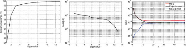
Figure 5.7: Analysis of the intrinsic dimensionality of the Cuprite scene by means of principal component analysis (PCA), minimum noise fraction (MNF), and the HySime method (right).

5.4.1 EXTRACTION TECHNIQUES

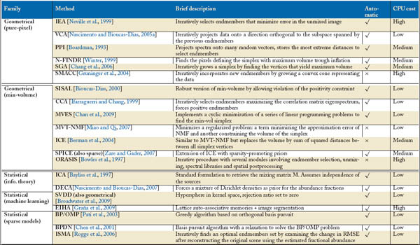
The previous step yields an estimated number of endmembers present in the scene by only looking at the statistical characteristics of the image. This number, however, could be known a priori in some specific cases where the area is well characterized. In those cases, manual methods for endmember extraction have been developed [Bateson and Curtiss, 1996, Tompkins et al., 1997]. However, this is not the case in many problems and hence automatic methods for endmember extraction are necessary. The problem can be casted as a blind source separation one because the sources and the mixing matrix are unknown. Even though ICA has been used to blindly unmix hyperspectral data [Bayliss et al., 1997, Chen and Zhang, 1999, Tu, 2000], its suitability to the problem characteristics has been questioned [Keshava et al., 2000, Nascimento and Bioucas-Dias, 2005b]. The main reason is that the assumption of mutual independence of the sources is not met by the problem in which abundances must sum to one. To solve the problems of ICA, many methods have been introduced. Two main families are identified: geometrical and statistical approaches [Parente and Plaza, 2010].

The family of geometrical methods consider the properties of the convex hull, and can be split into two subfamilies. The pure-pixel methods assume the presence of at least one pure pixel per endmember. This implies that there is at least one spectral vector on each vertex of the data simplex. This assumption limits the generality of the approaches but leads to very high computational efficiency. On the contrary, the family of minimum-volume methods estimate the mixing matrix M by minimizing the volume of the simplex. This is a nonconvex optimization problem much harder to solve. Geometrical methods can yield poor results when spectra are highly mixed. This is due to the lack of enough spectral vectors in the simplex facets.

Statistical methods can alleviate the above problems of geometrical methods, and constitute a very competitive alternative. In most of the cases, however, statistical methods have more computational burden. This family can be split into 1) methods based on information theory, such as ICA or the Dependent Component Analysis method (DECA), which assumes the abundance values are drawn from a Dirichlet distribution; 2) methods with inspiration in machine learning, such as the one-class SVM classifier that embraces all input samples in a feature spaces implicitly accessible via kernel functions (see Chapter 4) or associative neural networks; and 3) those that impose sparseness in the solution, such as the basis-projection denoising (BPDN) or the iterative spectral mixture analysis (ISMA).

Recently, a third approach based on sparse regression has been introduced [Iordache et al., 2011]. The main existing methods in all these families are summarized in Table 5.2. A more detailed description of the methods can be obtained from [Bioucas-Dias and Plaza, 2010, Plaza et al., 2011] and references therein.

5.4.2 A NOTE ON THE VARIBILITY OF ENDMEMBERS

A last important point to discuss regards the variability of endmembers. Spectral unmixing may give rise to unrealistic results because, even if algorithms succeed, the spectra representing the endmembers might not account for the spectral variability present in the scene. The issue of incorporating endmember variability in the spectral mixture analysis has been long studied and constitutes a crucial issue for the success of abundance estimation procedures [Bateson et al., 2000, García-Haro et al., 2005, Roberts et al., 1998]. Song [2005] reviewed how to incorporate endmember variability in the unmixing process for subpixel vegetation fractions in the urban environment. In [Settle, 2006] the effect of variable endmember spectra in the linear mixture model was studied. Selection of a meaningful set of free parameters and the inclusion of spatial information in the unmixing process have demonstrated useful for stabilizing the solution [García-Vílchez et al., 2011, Plaza and Chang, 2006].

5.4.3 A COMPARATIVE ANALYSIS OF ENDMEMBER EXTRACTION ALGORITHMS

This section compares several endmember determination methods representing different families: 1) pure-pixel geometrical approaches (IEA, VCA, PPI and NFINDR); 2) SISAL for geometrical minimum volume approaches; 3) ICA for the information-theoretic-based methods; and 4) SVDD target detection (see Section 4.4) and EIHA for the machine learning based approaches. To evaluate the goodness-of-fit of the extracted endmembers, we use different scores: the relative RMSE, the spectral angle mapper (SAM), and the spectral information divergence (SID). The SAM between and m is expressed as

The SID is an information-theoretic measure. Note that the probability distribution vector associated with each endmember signature is given by p = m/Σ_i m_i. Then, the similarity can be measured by the (symmetrized) relative entropy

Following the results of the previous section, 14 endmembers were extracted by the different techniques. Then, distances were computed between the endmembers extracted by each algorithm and the most similar ones in the USGS database m. This spectral library³ contains 501 cataloged spectra, so the search is a complex problem full of local minima. The signatures provided by each method were scaled by a positive constant to minimize the MSE between them and the corresponding library spectra for a proper comparison.

Figure 5.8 summarizes the performance of the methods in terms of computational cost, relative RMSE, SAM and SID angular errors. Regarding computational effort, the IEA, PPI and EIHA methods involve high computational burden. The rest of the methods are affordable for any current personal computer⁴. Regarding distance of the endmembers to those found in the database, all the methods achieve a relative RMSE lower than 0.2, except for PPI and ICA. Similar trends are observed for SAM and SID. The VCA outperformed the rest of the methods in accuracy (in all measures), and showed very good computational efficiency, closely followed by SVDD, SISAL and IEA. Particularly interesting is the case of the poor performance of ICA in terms of endmember extraction. The method is based on the assumption of mutually independent sources (abundance fractions), which is not the case of hyperspectral data since the sum of abundance fractions is constant, implying statistical dependence among them. Then, even if a basis is successfully extracted, the extracted endmembers by ICA do not necessarily have a physical (os spectra-like) shape because the problem is unconstrained. This is the main reason for the poor numerical results. Nevertheless, when used for synthesis, ICA may yield good results in terms of abundance estimation. More discussion on this issue can be obtained from [Nascimento and Bioucas-Dias, 2005b]. Another interesting issue is the good performance of the SVDD kernel method: in this case we fixed the rejection ratio to 0.001 (intuitively this reduces to embrace all data points in the kernel feature space) and the σ parameter for the RBF’s kernel was varied to give the requested p = 14. The method can be safely considered the best compromise between accuracy and computational cost among the statistical family, and constitutes a serious competitor to the pure geometrical methods. Actually, the SVDD can be considered a geometrical method with more flexibility to define the convex hull.

Figure 5.8: Computational cost (in secs.) and accuracy in terms of RMSE, SAM and SID for all the tested endmember extraction methods.

Looking at Fig. 5.9, the estimated signatures are close to the laboratory spectra. The bigger mismatches occur for 325 and 402 signatures for IEA and the SVDD, but only on particular spectral channels.

5.5 ALGORITHMS FOR ABUNDANCE ESTIMATION

The last step in spectral unmixing analysis consists in estimating the fractional abundances α. In the case that the basis is identified, the problem reduces to model inversion or regression approaches. Other approaches consider the steps of unmixing and abundance estimation jointly. We here review linear or nonlinear approaches found in the literature.

5.5.1 LINEAR APPROACHES

The class of inversion algorithms based on minimizing squared-error start from the simplest form of least squares inversion and increases in complexity as more constraints are included. The unconstrained least-squares problem is simply solved by = M^†r = (MM)⁻¹Mr. The issue of including the sum-to-one constraint means that the LS problem is constrained by Σα_i = 1, which can be solved via Lagrange multipliers. The non-negativity constraint is not as easy to address in closed-form as the full additivity. Nevertheless, a typical solution to the problem simply estimates iteratively and, at every iteration, finds a LS for only those coefficients of that are positive using only the associated columns of M. A fully constrained LS unmixing approach was presented in [Heinz and Chang, 2000]. The statistical analogue of least squares estimation minimizes the variance of the estimator. Under the assumption of additive noise, n, with covariance, C_n, the minimum variance estimate of the abundances reduces to This is called the minimum variance unbiased estimator (MVUE).

The number of algorithms for abundance estimation is ever-growing, and many variants and subfamilies are continuously being developed. In [Li and Narayanan, 2004], the use of features extracted after discrete wavelet transform improved the least squares estimation of endmember abundances. Abundance estimation of spectrally similar minerals by using derivative spectra in simulated annealing was presented in [Debba et al., 2006]. In [Chang and Ji, 2006], a weighted abundance-constrained linear spectral mixture analysis was successfully presented.

Miao et al. [2007] introduced the maximum entropy principle for mixed-pixel decomposition from a geometric point of view, and demonstrated that when the given data present strong noise or when the endmember signatures are close to each other, the proposed method has the potential of providing more accurate estimates than the popular least-squares methods. An updated revision of the available methods can be found in [Bioucas-Dias and Plaza, 2010].

5.5.2 NONLINEAR INVERSION

Due to the difficulties posed when trying to model the light interactions, the linear model has been widely adopted. Nevertheless, the model can be completed by plugging a nonlinear inversion method based on the estimated endmembers, either by exploiting the intimate spectral mixture to perform spectral unmixing or by definition of nonlinear decision classifiers. In this latter approach, multilayer perceptrons [Atkinson et al., 1997], nearest neighbor classifiers [Schowengerdt, 1997], and support vector machines (SVMs) [Brown et al., 2000] have been used. Actually, the nonlinear extensions via kernels allow SVMs to deal with overlapping pure pixels distributions and nonlinear mixture regions. Adopting a linear model while performing nonlinear decision boundaries can be done in a feature space via a nonlinear reproducing kernel function [Camps-Valls and Bruzzone, 2009]. See Chapters 4 and 4 for discussion on kernel nonlinear feature extraction and classification, respectively. Following this idea, nonnegative constrained least squares and fully constrained least squares in [Harsanyi and Chang, 1994] were extended to their kernel-based counterparts [Broadwater et al., 2009]. A simple algorithm for doing nonlinear regression with kernels consists of iterating the equations:

= (K(M, M))⁻¹ [K(M, r) − λ]

λ = K(M, r) − K(M, M),          

Figure 5.9: Comparison of the extracted signatures (blue) with those in the USGS spectral library (red) for a representative method of each family: IEA (geometrical, pure-pixel), VCA (geometrical, minimum-volume) and SVDD (statistical).

where λ is the Lagrange multiplier vector used to impose the non-negativity constraints of the estimated abundances. Nevertheless, the method does not incorporate the sum-to-one constraint. We refer to this method as the Kernel NonNegativity Least Squares (KNNLS).

5.5.3 A COMPARATIVE ANALYSIS OF ABUNDANCE ESTIMATION ALGORITHMS

We here compare LS and KNNLS methods for abundance estimation. For the sake of brevity, we only apply the methods to the endmembers identified by the VCA method, which gave the best overall results. Figure 5.10 illustrates the estimated abundance maps. The obtained maps nicely resemble the available geological maps. In general, both linear and nonlinear methods yield similar results. Nevertheless, for some particular cases, the use of the KNNLS achieves more detailed description of the spatial coverage (see e.g., minerals 386 and 245) or less noisy maps (see e.g., minerals 126, 139, and 299). The main problem with KNNLS in this case is the proper tuning of the σ parameter for the kernels, which we fixed to the sample mean distance between pixels. Another critical issue is that the model does not include the sum-to-one constraint in a trivial way. Nevertheless, there are versions of KNNLS to include them [Broadwater et al., 2009].

5.6 SUMMARY

This chapter reviewed the field of spectral mixture analysis of remote sensing images. The vast literature has been revised in terms of both applications and theoretical developments. We observed tight relations to other fields of signal processing and statistical inference: very often, terms like ‘domain description’, ‘convex hull’, or ‘nonlinear model inversion with constraints’ appear naturally in the field. The problem is highly ill-posed in all steps, either when identifying the most representative pixels in the image or when inverting the mixing model. These issues pose challenging problems. Currently, quite efficient methods are available, which has led to many real applications, mainly focused on identifying crops and minerals to finally deploy abundance (probability) maps. All steps in the processing chain were analyzed and motivated theoretically and also tested experimentally.

Figure 5.10: Abundance maps of different minerals estimated using least squares linear unmixing (top panel) and the kernel version (bottom panel) for the VCA method. The different materials identifiers in the USGS report are indicated above.

¹http://aviris.jpl.nasa.gov/html/aviris.freedata.html

²http://speclab.cr.usgs.gov/spectral-lib.html

³Very often we are aware of the type of class we are looking for. In this case, we may have some labeled pixels of the class of interest or we can rely on databases (often called spectral libraries) of class-specific spectral signatures. In this case, the problem reduces to defining the background class and then detecting spectral signatures that are closer to the known signatures than to the background.

⁴All experiments were carried in Matlab usinga2GbRAM,2 processors, 3.3 GHz CPU station.