
Classification of Remote Sensing Images
The advances in remote sensing sensors (see Chapter 1) allow description of the objects of interest with improved spatial and spectral resolutions. The excellent quality in the acquired data gives rise at the same time to challenging problems for automatic image classification1. This chapter considers these challenges. First, we present different classification problems that benefit from the use of remote sensing data and briefly present the solutions considered in the field. After the definition of the classification problem (Section 4.1.1), the main classification tasks will be presented in sections 4.2 to 4.4. Finally, Section 4.5 discusses the new challenges to be confronted in these fields, including representativeness and adaptation of classifiers.
4.1 INTRODUCTION
Classification maps are one of the main products for which remote sensing images are used. The specific application may differ, but the general aim is to associate the acquired spectra to a limited number of classes. These classes are expected to facilitate the description or detection of objects at the Earth’s surface. In the context of decision making, classification maps are useful, because they summarize the complex spatial-spectral information into a limited number of classes of interest.
4.1.1 THE CLASSIFICATION PROBLEM: DEFINITIONS
Consider a task such as distinguishing different soil types using their spectral signature, or discerning trees from buildings using aerial photography. All these problems share the task of predicting a class membership (or label) yi ∈ ![]() from a set of d-feature samples
from a set of d-feature samples ![]() The labels correspond to different classes, whose nature is specific to each applicative domain. The features are typically the spectral bands of a satellite/airborne image (for instance, x = {x(1) = blue band, x(2) = green band, x(3) = red band, x(4) = near infrared band}
The labels correspond to different classes, whose nature is specific to each applicative domain. The features are typically the spectral bands of a satellite/airborne image (for instance, x = {x(1) = blue band, x(2) = green band, x(3) = red band, x(4) = near infrared band}![]() ), spatial or contextual features extracted over some specific channels, or full hyperspectral patches. See Chapters 2 and 3 for details about these families of features. The variables (or features hereafter) included in x are supposed to be discriminative for the classification task. Figure 4.1 shows a generic flowchart of remote sensing image classification. Given the set of d features, two main schemes are adopted:
), spatial or contextual features extracted over some specific channels, or full hyperspectral patches. See Chapters 2 and 3 for details about these families of features. The variables (or features hereafter) included in x are supposed to be discriminative for the classification task. Figure 4.1 shows a generic flowchart of remote sensing image classification. Given the set of d features, two main schemes are adopted:
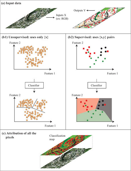
Figure 4.1: General remote sensing image classification problem.
• Unsupervised classification (Fig. 4.1(b1)), where the features are used to identify coherent clusters in the data distribution. The aim of such methods is to split the data into groups as similar as possible, without knowing the nature of such groups.
• Supervised classification (Fig. 4.1(b2)) refers to the situation in which a series of input-output pairs (the training set) are available and used to build a model. The model learns a function to assign output labels (or targets) to every input feature vector using the training set. In most settings, training data are assumed to be representative of the whole data distribution and to be independent and identically distributed (i.i.d.). We will come back about this statement in Section 4.5.5.
In both cases, a model with Θ parameters ![]() = f(x, Θ) is constructed using the training data x and then applied to the entire image, in order to have the class estimate
= f(x, Θ) is constructed using the training data x and then applied to the entire image, in order to have the class estimate ![]() of each pixel in the image. The main difference for the application of one of these approaches resides in the availability of training labels.
of each pixel in the image. The main difference for the application of one of these approaches resides in the availability of training labels.
4.1.2 DATASETS CONSIDERED
In all the experiments presented in this chapter, two QuickBird images of Brutisellen –a residential neighborhood of Zürich, Switzerland– have been used to assess the performance of the algorithms presented. The images have been acquired in August 2002 and October 2006, respectively, and have a spatial resolution of 2.4 m. They are coregistered, 4-dimensional (Near Infrared, Red, Green and Blue bands) and with an extent of 329 × 347 pixels. A total of 40762 (2002 image) and 28775 (2006 image) pixels were labeled by photointerpretation and belong to 9 land-use classes. Figure 4.2 illustrates the images and the labeled pixels available. For each application, the nature of the outputs has been defined in the corresponding section.
In addition, we evaluate the performance of semisupervised algorithms in an AVIRIS image acquired over the Kennedy Space Center (KSC), Florida, on 1996, with a total of 224 bands of 10 nm bandwidth with center wavelengths from 400-2500 nm. The data was acquired from an altitude of 20 km and has a spatial resolution of 18 m. After removing low SNR bands and water absorption bands, a total of 176 bands remains for the analysis. The dataset originally contained 13 classes representing the various land cover types of the environment, containing many different marsh subclasses that we decided to merge them in a fully representative marsh class. Thus, we finally used 10 classes: ‘Water’ (761), ‘Mud flats’ (243), ‘Marsh’ (898), ‘Hardwood swamp’ (105), ‘Dark/broadleaf’ (431), ‘Slash pine’ (520), ‘CP/Oak’ (404), ‘CP Hammock’ (419), ‘Willow’ (503), and ‘Scrub’ (927). The image can be downloaded from http://www.csr.utexas.edu/.
4.1.3 MEASURES OF ACCURACY
Classification accuracy is typically evaluated on a test set independent from the training set, in order to assess generalization capabilities of the models. Several standard quality measures in the remote sensing literature are commonly used.
Overall accuracy The overall accuracy (OA) is the number of pixels correctly classified divided by the total number of test pixels: this measure shows the ratio between correct labels and commission errors, i.e., the pixels attributed to a wrong class.
Kappa index The overall accuracy can be a misleading index, since several correct classifications may occur by chance. Very often the estimated Cohen’s Kappa statistic κ is preferred instead [Foody, 2004]. This index is computed by comparing the number of pixels classified correctly by the model to the number of pixels classified correctly by random chance.

Figure 4.2: Images used in the experiments: Images of Brutisellen (Zürich, Switzerland) and corresponding ground surveys. Subfigures (a-b) show the 2002 image, while subfigures (c-d) show the 2006 image. Subfigures (e) and (f) illustrate the classes used for the change detection experiments: in panel (e), the changed and unchanged areas are highlighted in black and grey, respectively; panel (f) shows the color code used in Figure 4.4 (yellow = soil to buildings; cyan = meadows to building; light pink = soil to vegetation; dark pink = vegetation to road).
Mean tests In the case of multiple experiments reported in this survey, a mean test is used to see if the mean Kappa for the first model, ![]() 1, is significantly higher than the mean kappa obtained by the second model,
1, is significantly higher than the mean kappa obtained by the second model, ![]() 2. We thus use the standard formulation for a mean test statistic for two populations. We reject the hypothesis of
2. We thus use the standard formulation for a mean test statistic for two populations. We reject the hypothesis of ![]() 1 being less or equal to
1 being less or equal to ![]() 2 if and only if
2 if and only if

where s1 and s2 are the observed standard deviations for the two models, n1 and n2 are the number of realizations of experiments reported and t1−α is the α-th quantile of the Student’s law (typically α = 0.05 is used).
McNemar’s test The McNemar’s test [Foody, 2004], or Z-test, is a procedure used for assessing the statistical difference between two maps when the same samples are used for the assessment. It is a nonparametric test based on binary confusion matrices. The test is based on the z statistic:
![]()
where fij indicates the number of pixels in the confusion matrix entry (i, j). This index can be easily adapted to multiclass results by considering correct (diagonal) and incorrect (off-diagonal) results. When z is positive (or, in accordance to 95-th quantile of the normal law ![]() (0, 1), greater than 1.96), the result of the second map can be considered as statistically different. When |z| < 1.96, the maps cannot be considered as statistically significantly different, and when z is negative, the first result statistically outperforms the second one.
(0, 1), greater than 1.96), the result of the second map can be considered as statistically different. When |z| < 1.96, the maps cannot be considered as statistically significantly different, and when z is negative, the first result statistically outperforms the second one.
ROC curves In problems involving a single class, such as target detection (see Section 4.4), the receiver operating characteristic (ROC) curve is used to compare the sensitivity of models. By sensitivity, we mean the relation between the true positive rate (TPR) and the false positive rate (FPR). These two measures define the first and second type risk, respectively. In the experiments of Section 4.4, we use a traditional measure computed from the ROC curve, the Area Under the Curve (AUC): this area can be interpreted as the probability that a randomly selected positive instance will receive a higher score than a negative instance.
4.2 LAND-COVER MAPPING
Land-cover maps are the traditional outcome of remote sensing data processing. Identifying specific land cover classes on the acquired images may help in decision-making by governments and public institutions. The land-cover maps constitute an important piece to complement topographic maps, agriculture surveys, or city development plans, which are fundamental for decision-making and planning. Traditionally, these maps are retrieved by manual digitalization of aerial photography and by ground surveys. However, the process can be automatized by using statistical models as the ones illustrated in Fig. 4.1. Land-cover classification problems can be resumed to the task of classifying an image using information coming from this same image. The outputs represent a series of land-cover classes, for instance y = {1: vegetation, 2: man-made, 3: soil}. In the following, the application of supervised and unsupervised methods to remote sensing images is briefly summarized (cf. Fig. 4.1).
4.2.1 SUPERVISED METHODS
The contribution of supervised methods has been improving the efficacy of the land-cover mapping methods since the 1970s: Gaussian models such as Linear Discriminant Analysis (LDA) were replaced in the 1990s by nonparametric models able to fit the distribution observed in data of increasing dimensionality. Decision trees [Friedl and Brodley, 1997, Hansen et al., 1996] and then more powerful neural networks (NN, Bischof and Leona [1998], Bischof et al. [1992], Bruzzone and Fernández Prieto [1999]) and support vector machines (SVM, Camps-Valls and Bruzzone [2005], Camps-Valls et al. [2004], Foody and Mathur [2004], Huang et al. [2002], Melgani and Bruzzone [2004]) were gradually introduced in the field, and quickly became standards for image classification. In the 2000s, the development of classification methods for land-cover mapping became a major field of research, where the increased computational power allowed 1) to introduce different types of information simultaneously and to develop classifiers relying simultaneously on spectral and spatial information [Benediktsson et al., 2003, 2005, Fauvel et al., 2008, Pacifici et al., 2009a, Pesaresi and Benediktsson, 2001, Tuia et al., 2009a], 2) the richness of hyperspectral imagery [Camps-Valls and Bruzzone, 2005, Plaza et al., 2009], and 3) exploiting the power of clusters of computers [Muñoz-Marí et al., 2009, Plaza et al., 2008].
Kernel methods were the most studied classifiers: ensembles of kernels machines [Briem et al., 2002, Waske et al., 2010], fusion of classification strategies [Bruzzone et al., 2004, Fauvel et al., 2006, Waske and J. A. Benediktsson, 2007] and the design of data-specific kernels –including combinations of kernels based on different sources of information [Camps-Valls et al., 2006b, Tuia et al., 2010a,c] or spectral weighting [Baofeng et al., 2008]– became major trends of research and attracted the increasing interest from users and practitioners.
4.2.2 UNSUPERVISED METHODS
Although less successful than supervised methods, unsupervised classification is still attracting a large consensus in remote sensing research. The problem of the acquisition of labeled examples makes unsupervised methods attractive and thus ensure constant developments in the field2. Two main approaches to unsupervised classification for land-cover mapping are found in the literature: partitioning methods, that are techniques that split the feature space into distinct regions, and hierarchical methods, that return a hierarchical description of the data in the form of a tree or dendrogram.
Partitioning methods are the most studied in remote sensing: first, fuzzy clustering has been used in conjunction with optimization algorithms to cluster land-cover regions in Maulik and Bandyopadhyay [2003] and Maulik and Saha [2009]. This approach is extended to multiobjective optimization in [Bandyopadhyay et al., 2007] where two opposing objective functions favoring global and local partitioning were used to enhance contextual regularization. Other regularization strategies include the fusion of multisource information [Bachmann et al., 2002, Sarkar et al., 2002] or rule-based clustering [Baraldi et al., 2006]. Graph cuts have been reconsidered more recently [Tyagi et al., 2008] where the authors proposed a multistage technique cascading two clustering techniques, graph-cuts and fuzzy c-means, to train the expectation-maximization (EM) algorithm. The use of self organizing maps is proposed in [Awad et al., 2007]. Tarabalka et al. [2009] use ISOMAP to regularize the SVM result by applying a majority vote between the supervised and the unsupervised method.
Hierarchical methods cluster data by iteratively grouping samples according to their similarity using typically an Euclidean distance. The relevance of this family of algorithms has been reported in a variety of remote sensing applications, including delimitation of climatic regions [Rhee et al., 2008], identification of snow cover [Farmer et al., 2010], characterization of forest habitats [Bunting et al., 2010] or definition of oceanic ecosystems [Hardman-Mountford et al., 2008]. For specific tasks of image segmentation, spatial coherence of the segments is crucial. Therefore, contextual constraints have been included into the base algorithms. As an example, multistage restricted methods are proposed in [Lee, 2004, Lee and Crawford, 2004] to perform first a region growing segmentation to ensure spatial contiguity of the segments, and then to perform classical linkage to merge the most similar segments. In [Marcal and Castro, 2005], several informative features are included in the aggregation rule: spatial criteria accounting for cluster compactness, cluster size, and the part of their boundaries that two clusters share ensure spatially coherent clusters. Fractal dimension is used as a criterion of homogeneity in [Baatz and Schäpe, 2000]. Other ways to ensure spatial coherence is to use region-growing algorithms: Tarabalka et al. [2010] utilize random forests for that purpose. Watershed segmentation on the different resolutions is proposed in [Hasanzadeh and Kasaei, 2010], where it is used in conjunction with fuzzy partitioning to account for connectedness of segments.
4.2.3 A SUPERVISED CLASSIFICATION EXAMPLE
In the following we provide a comparison of five supervised methods for land-use mapping in an urban environment. The compared methods are LDA, a standard classification tree, k-nearest neighbors, SVM, and the multilayer perceptron. Urban areas are the most challenging problems in very high resolution image classification because they present a great diversity and complexity in the objects represented [Licciardi et al., 2009b]. In particular, the geometry and context that can be retrieved is essential to account for different land uses that are composed by the same material (thus the same spectral behavior at the pixels level) but vary as a function of its context.
To stress this point, Tables 4.1 and 4.2 show the numerical results obtained by the methods with and without contextual features on the QuickBird image of Brutisellen (Switzerland) described in Section 4.1.2. For the nine classes of interest, small differences can be made between classes ‘Roads’ and ‘Parkings’ (both are asphalt) and between ‘Trees’ and ‘Meadows’. To enhance the performance in these classes, morphological top-hat features (see Chapter 3) have been computed for the four bands and stacked to the multispectral bands before training the classifiers.
The numerical results show a few clear trends: the excellent performances of nonparametric methods such as support vector machines and neural networks, the good performance of lazy learners as k-nearest neighbors when a sufficient number of labeled examples is available, and the poor performance of linear parametric classifiers as the LDA. The addition of contextual information is beneficial for all models, whose accuracy increases between 5% and 10%. Interestingly, note that without contextual information, SVM and NN are statistically inferior to k-NN, because they attempt to generalize classes that cannot be separated with spectral information only. On the other hand, k-NN outperforms the other methods when using non-discriminative information, since the model does not rely on a trained model and analyzes each pixel by its direct neighbors.
The classification maps obtained with the different approaches with contextual information are illustrated in Fig. 4.3: among all classifiers presented, SVM and k-NN return the closest maps to the expected result, and can efficiently detect all major structures of the image. This demonstrates the suitability of nonparametric models for supervised image classification. For this realization, the MacNemar’s test confirmed these visual estimation of the quality: SVM map is significantly better than the others, followed by the k-NN and NN maps.
Table 4.1: Comparison of supervised classification algorithms. Mean overall accuracy and Kappa statistics (see Section 4.1.3), along with standard deviation of five independent experiments. In bold, the best performing method. Underlined, results with average Kappa statistically inferior to the best method.
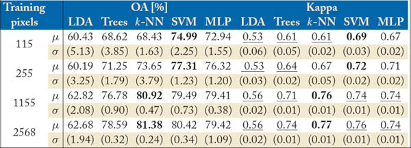
Table 4.2: Comparison of supervised classification algorithms with contextual information. Mean overall accuracy and Kappa statistics (see Section 4.1.3), along with standard deviation of five independent experiments. In bold, the best performing method. Underlined, results with average Kappa statistically inferior to the best method.


Figure 4.3: Classification maps of the experiments using contextual information and 1155 training pixels. Best results are shown in parentheses in the form of (OA [%], κ).
4.3 CHANGE DETECTION
The second family of classification problems discussed in this chapter is related to the detection of class transitions between a pair of co-registered images, also known as change detection [Radke et al., 2005, Singh, 1989]. Change detection is attracting an increasing interest from the application domains, since it automatizes traditionally manual tasks in disaster management or developments plans for urban monitoring. We should also note that multitemporal classification and change detection are very active fields nowadays because of the increasing availability of complete time series of images and the interest in monitoring Earth’s changes at local and global scales. In a few years from now, complete constellations of civil and military satellites sensors will deliver a much higher number of revisit time images. To name a few, the ESA’s Sentinels3 or NASA’s A-train4 programs are expected to produce near real-time scientific coverage of the globe in the next decades.
Three types of products are commonly studied in the change detection framework [Coppin et al., 2004, Singh, 1989]: binary maps, detection of types of changes and full multi-class change maps, thus including classes of changes and unchanged land-cover classes. Each type of product can be achieved using different sources of information retrieved from the initial spectral images at time instants t1 and t2. Therefore, the input vector x can be either composed by both separate datasets x(1) and x(2), or by a combination of the features of two images taken at time instants t1 and t2. Singh [1989] underlines that changes are likely to be detected if their changes in radiance are larger than changes due to other factors such as differences in atmospheric conditions or sun angle. Many data transformations have been used to enhance the detection of changes:
• the stacking of feature vectors xstack = [x(1), x(2)], mainly used in supervised methods,
• the difference image xdiff = |x(1) – x(2)|, where unchanged areas show values close to zero,
• image ratioing ![]() where unchanged areas show values close to one,
where unchanged areas show values close to one,
• data transformations as principal components (see Chapter 3), where changes are grouped in the components related to highest variance,
• physically based indices as NDVI (see Chapters 3 and 6), useful to detect changes in vegetation.
However, these transforms do not cope with problems of registration noise or intraclass variance. Therefore, algorithms exploiting contextual filtering (see Chapter 3) have been also considered in the literature. In the following section, a brief review of different strategies is reported.
4.3.1 UNSUPERVISED CHANGE DETECTION
Unsupervised change detection has been widely studied, mainly because it meets the requirements of most applications: i) the speed in retrieving the change map and ii) the absence of labeled information. However, the lack of labeled information makes the problem of detection more difficult and thus unsupervised methods typically consider binary change detection problems. To do so, the multitemporal data are very often transformed from the original to a more discriminative domain using feature extraction methods, such as PCA or wavelets, or converting the difference image to polar coordinates, i.e., magnitude and angle. In the transformed space, radiometric changes are assessed in a pixel-wise manner.
The most successful unsupervised change detector until present remains the change vector analysis (CVA, [Bovolo and Bruzzone, 2007, Malila, 1980]): a difference image is transformed to polar coordinates, where a threshold discriminates changed from unchanged pixels. In [Dalla Mura et al., 2008], morphological operators were successfully applied to increase the discriminative power of the CVA method. In [Bovolo, 2009], a contextual parcel-based multiscale approach to unsupervised change detection was presented. Traditional CVA relies on the experience of the researcher for the threshold definition, and is still on-going research [Chen et al., 2010a, Im et al., 2008]. The method has been also studied in terms of sensitivity to differences in registration and other radiometric factors [Bovolo et al., 2009].
Another interesting approach based on spectral transforms is the multivariate alteration detection (MAD, [Nielsen, 2006, Nielsen et al., 1998]), where canonical correlation is computed for the points at each time instant and then subtracted. The method consequently reveals changes invariant to linear transformations between the time instants. Radiometric normalization issues for MAD has been recently considered in [Canty and Nielsen, 2008].
Clustering has been used in recent binary change detection. In [Celik, 2009], rather than converting the difference image in the polar domain, local PCAs are used in subblocks of the image, followed by a binary k-means clustering to detect changed/unchanged areas locally. Kernel clustering has been studied in [Volpi et al., 2010], where kernel k-means with parameters optimized using an unsupervised ANOVA-like cost function is used to separate the two clusters in a fully unsupervised way.
Unsupervised neural networks have been considered for binary change detection: Pacifici et al. [2009b] proposed a change detection algorithm based on pulse coupled neural networks, where correlation between firing patterns of the neurons are used to detect changes. In [Pacifici et al., 2010], the system is successfully applied to earthquake data. In Ghosh et al. [2007], a Hopfield neural network, where each neuron is connected to a single pixel is used to enforce neighborhood relationships.
4.3.2 SUPERVISED CHANGE DETECTION
Supervised change detection has begun to be considered as a valuable alternative to unsupervised methods since the advent of very high resolution (VHR) sensors made obtaining reliable ground truth maps by manual photointerpretation possible. Basically, two approaches are found in the literature: the post-classification comparison (PCC, [Coppin et al., 2004]) and the multitemporal classification [Singh, 1989], which can be roughly divided into direct multi-date classification and difference analysis classification. The next paragraphs review these two approaches.
PCC methods are based on individual classifications of the datasets at each time instant. Once the classification maps are obtained, the results are computed by subtracting them. Traditional PCC is often inefficient because it suffers from the cumulation of the errors made by individual classifications. This ends up in salt-and-pepper change detection maps, where several changes in unchanged areas (typically at the borders between classes) are observed. Purple areas in Fig. 4.4(a) are areas where these errors occur. To cope with these errors, postclassification masking has been proposed in [Pacifici et al., 2007]: a neural network trained to solve a binary change vs. no-change problem masks the unchanged areas, thus decreasing the post-classification errors. In [Chen et al., 2010a], CVA is used for this same purpose and also for discriminating the type of changes. Although very efficient, these approaches consider consequences rather than causes of the PCC problems.
Multitemporal classification has been considered in three settings: by using stacked vectors xstack before training the classifier (DMC), by computing a difference image xdiff before analysis (DIA), or by designing classifier-specific measures to cope for both time instants simultaneously. The main difference between the two first is that DMC can return a full land-cover change maps, where both the changed and unchanged land-cover types are described, while DIA cannot differentiate among unchanged land-cover types, as they all reduce to spectra with nearly null components. Regarding the third setting, Camps-Valls et al. [2008a] studied the effect of summation, difference and ratio kernels to solve change detection problems with binary, multiclass and one-class SVM. In this work, the use of composite kernels also allows one to combine information from different time instants and multisource images (e.g., optical and radar images). Actually, we should note that the use of spatial and contextual features is currently poorly documented in supervised change detection. Only few studies can be found (see, for instance, Pagot and Pesaresi [2008], Volpi et al. [2011a]). However, they all confirm the interest of filtering the magnitude of the difference image to reduce radiometric differences and registration errors.

Figure 4.4: Supervised change detection results. (a) PCC (purple areas are misclassified areas, where unobserved transitions are detected); (b) DMC stacked multiclass; (c) SVM with summation kernel (SVM specific); (d) DIA; (e) DMC stacked without differences in the unchanged class; (f) SVM with summation kernel without differences in unchanged areas. Best results are shown in parentheses in the form of (OA [%], κ).
Finally, the scarceness of labeled examples has been tackled with target detection models [Camps-Valls et al., 2008a] and semisupervised learning [Bovolo et al., 2008, Gómez-Chova et al., 2010, Muñoz-Marí et al., 2010]. These two aspects will be detailed in Sections 4.5.1 and 4.4, respectively.
4.3.3 A MULTICLASS CHANGE DETECTION EXAMPLE
In this section, four approaches for supervised change detection are compared for the VHR image of Brutisellen, described in Section 4.1.2. In particular, we used PCC, DMC, SVM with summation kernel [Camps-Valls et al., 2008a] and DIA in two settings: multiclass change detection (PCC, DMC and SVM) and detection of types of changes (DIA, DMC and SVM). The same contextual information as in the classification example has been used, and four classes of change have been considered, as illustrated in Fig. 4.2(f): meadows to buildings, soil to buildings, meadows to roads and soil to meadows. The change detection results are illustrated in Fig. 4.4.
The change detection maps of Fig 4.4 confirm the main disadvantage of PCC: many false alarms are detected (in purple in Fig 4.4(a)) since they correspond to single classification errors and differences in object borders. Both DMC and SVM with summation kernels (a weighted sum of kernels specialized in describing similarities at time instants t1 and t2) solve this problem and return land-use maps accounting for the changes that have occurred between the two dates. DMC seems more dependent on the registration noise (see, for instance, the path in the middle of the meadow on the left side of the image). The summation kernel can better exploit the specific spatial context of the pixels and reduces the misclassification rate, mainly due to the fact that estimates similarities separately for each time instant.
Considering the detection of types of changes, the three algorithms detect the main patches of change in the image. However, DIA returns a noisy result since it is based on a difference image and nonzero vectors may be erroneously interpreted as change. On the contrary, DMC and even more the summation kernel return improved description of the unchanged class, while losing precision in the description of the changed classes. According to the analyst’s interest (detecting clearly changed areas or fine detection of type of changed objects), DIA or SVM with specialized kernels should be the preferred methods in this problem.
4.4 DETECTION OF ANOMALIES AND TARGETS
This section is devoted to the field of automatic target detection. Some applications relying on remote sensing data do not need the definition of many classes of interest. Actually, very often, they only need to discriminate a single class from the rest, i.e., the background [Ahlberg and Renhorn, 2004]. Sometimes, there is no knowledge about the signature of the class of interest, but it is known that this signature is different from the rest. In this case, a model is built by looking for signatures that deviate from a model of the background. Large deviations from the mean are called anomalies, and the models based on this principle are referred to as anomaly detectors. Anomaly detectors can be very difficult to calibrate, especially when there is a strong spectral variability in the image. This field is related to the identification of endmembers that will be treated in Chapter 5.
Most of the time we are aware of the type of class we are looking for. In this case, we may have some labeled pixels of the class of interest or we can rely on databases (often called spectral libraries) of class-specific spectral signatures. In this case, the problem reduces to defining the background class and then detecting spectral signatures that are closer to the known signatures than to the background. Algorithms searching for these signatures, or targets, are referred to as target detectors. Target detection is of particular interest when the targets are subpixel targets or buried objects, thus known but difficultly detectable on the image [Chang, 2003, Chang and Heinz, 2000]. Subpixel target detection, or unmixing will be detailed in Chapter 5. In the rest of this chapter, we will consider anomalies and targets bigger than a pixel. Table 4.3 summarizes the anomaly and target detection methods presented in the next sections.
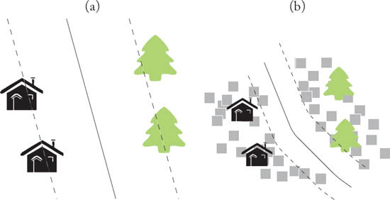
Figure 4.5: Semisupervised learning: (a) the model obtained with the labeled samples only is not representative of the global probability density function (PDF). (b) By integrating the PDF statistics, the model adapts to the unlabeled data.
Table 4.3: Taxonomy of anomaly and target detectors (adapted from Ahlberg and Renhorn [2004] and Kwon and Nasrabadi [2007a]).

4.4.1 ANOMALY DETECTION
When the signature of the class to be detected is unknown, anomaly detection algorithms are used. Anomaly detection reduces to assuming (and/or defining) a model for the background class, and then looks for the test samples lying far from the mean of the background distribution.
Depending on the assumptions made on the background, different anomaly detectors can be used. If the background is modeled as a Gaussian distribution, the Reed-Xiaoli (RX) [Lu et al., 1997, Reed and Yu, 1990] detector can be used. The RX detector detects outliers by computing a Mahalanobis distance between the considered pixel and the background mean vector. If the background is believed to be more complex, for instance multi-Gaussian, it can be modeled with a Gaussian mixture model [Beaven et al., 2000]. Application of these principles to the detection of small objects in series of remote sensing images can be found in [Carlotto, 2005]. More recently, the RX detector has been extended to its nonlinear kernelized version in [Kwon and Nasrabadi, 2005].
Another possibility is to model the background as a linear subspace described by a set of linearly independent basis vectors. Assuming such a model, any vector in the subspace can be written as a linear combination of these basis functions. As seen before, these basis functions are known in remote sensing as endmembers. The Distance From Feature Space (DFFS) detector computes the distance of the pixel from the background as the squared norm of the residual among the pixel and its projection in the linear subspace. Kernel PCA has been used in [Gu et al., 2008] to project data into a nonlinearly independent space: the RX algorithm is then successfully applied on the component maximizing a measure of skewness and kurtosis.
If no global assumptions are made and one assumes that only local samples are important, nearest neighbor detectors can be used instead. In this case, the distance of the pixels to their nearest neighbors in the background are computed: the weighted mean distance is then thresholded to decide whether the pixel is an outlier or not. Finally, nonparametric models can be used to model the background, as in [Banerjee et al., 2009], where a support vector domain description (SVDD) is used to model the background and then detect outliers, which are the pixels lying outside the region of support of the background pixels. We will use this model in Section 5.4.
Another recent field of investigation in this direction is anomalous change detection [Theiler, 2008b]: in this field, one looks for changes that are interestingly anomalous in multitemporal series, and tries to highlight them in contrast to acquisition condition changes, registration noise, or seasonal variation [Theiler et al., 2011]. Methods span from chronochrome maps [Schaum and Stocker, 1997a,b], where the best linear estimator for the background in the second time instant is found, to covariance equalization methods [Schaum and Stocker, 1994], methods estimating the mutual information between the appearance of given values in the two acquisitions [Theiler and Perkins, 2006] and pervasive methods [Theiler, 2008a], where noise is added to an image to account for misregistration.
4.4.2 TARGET DETECTION
When the target is partially or entirely known, this additional knowledge can be used to design more accurate target detectors: rather than assessing the distance from a background distribution, the pixel is compared against target and background and then assigned to the closest class.
When the background and target are assumed to be Gaussian-distributed, a likelihood function can be used to decide whether a pixel belongs to one or the other. Such likelihood maximizes the distance to the background and minimizes the distance to the target simultaneously. Using a Mahalanobis distance, this target detector is called the adaptive matched filter (AMD). Another possibility is to use the spectral angle mapper (SAM) as a measure of distance. Such measure assesses the angle between the target and the pixel to be evaluated with a dot product.
When using a linear subspace for the background model, the orthogonal space projection (OSP) detector is one of the most famous models used in remote sensing [Lu et al., 1997, Reed and Yu, 1990]: in this case, the subspace of the background basis functions is removed from the analyzed pixel, thus leaving only the part related to the target signature. This reduced spectral signature is then matched with the target signature: if the match exceeds a given threshold, the pixel is considered as target. OSP detectors have been extended to the nonlinear case using kernel methods in [Kwon and Nasrabadi, 2005]: the kernel orthogonal space projection (KOSP) calculates the OSP detector in a high dimensional feature space and can handle non-Gaussian complex background models. In [Capobianco et al., 2009], a semisupervised version of KOSP is proposed using graphs to preserve the structure of the manifold (the field of semisupervised learning was treated in Section 4.5.1). Other popular linear target detection approaches include the matched subspace detector (MSD) [Scharf and Friedlander, 1994], the spectral matched filter (SMF) [Robey et al., 1992], and the adaptive subspace detectors (ASD) [Kraut et al., 2001]: Kwon and Nasrabadi [2007a] present a review on these target detectors and their kernel counterparts: see kernel matched subspace detector (KMSD Kwon and Nasrabadi [2006b]), kernel spectral matched filter (KSMF Kwon and Nasrabadi [2007b]) and kernel adaptive subspace detector (KASD Kwon and Nasrabadi [2006a]). Other methods that project data into an orthogonal low-dimensional space can be used to separate target from background: principal components analysis, Fisher’s discriminant and eigenspace separation, along with their kernel counterparts can be used for this purpose [Nasrabadi, 2009].
Another possibility is to reduce the target detection problem to a single class classification problem. Nonparametric methods, such as SVDD [Muñoz-Marí et al., 2007] and the one-class SVM [Camps-Valls et al., 2008a, Muñoz-Marí et al., 2010, Wang et al., 2006] can also be used for target detection: in this case, the known target pixels are used to train the model. A traditional application for this type of approach is the detection of landmines: among others, contextual-aware approaches such as Hidden Markov Models [Gader et al., 2001, Zhu and Collins, 2005], 3-D histograms [Frigui and Gader, 2009], random sets [Bolton and Gader, 2009] and multiple instance learning [Bolton and Gader, 2010] have been proposed for this purpose.
4.4.3 A TARGET DETECTION EXAMPLE
In the following, four target detectors are compared in the task of detecting the class ‘Soil’ of the Zürich image. In Figs. 4.6(a)-(d), the detections of OSP and KOSP with varying parameters are illustrated. OSP returns a decision function strongly contaminated by noise, and it is difficult to apply a threshold to efficiently isolate the target. On the contrary, a well-calibrated KOSP detector can result into correct detection, as shown in Fig. 4.6(c). However, KOSP appears as being strongly influenced by the choice of the kernel parameter: a too small σ results in overfitting the target endmember signature (Fig. 4.6(b)), while a too large kernel bandwidth σ returns a completely wrong detection (Fig. 4.6(d)).

Figure 4.6: Comparison of algorithms for target detection of the class ‘Soil’ (in brown): values of the discriminative function for (a) OSP, (b-d) KOSP with different kernel parameters, (e) SAM detector and (f) One class SVM using 50 pixels representing the target. Kappa is maximized by varying the detection threshold.
The SAM detector returns a good reconstruction of the target, but with strong false alarms in the bottom left side of the image, where the roof of the commercial center saturates the sensor and thus returns a flat spectrum for its pixels in the morphological features. As a consequence, both the target and the roof vectors have flat spectra and their spectral angle is almost null. The one-class SVM returns a highly discriminative function, where the target and background are nicely discriminated. The rate of false alarms is thus minimized, returning the best numerical and visual result among the compared methods.
This section deals with emerging problems in remote sensing image classification. Now that the methodologies have reached a great degree of sophistication and precision, new problems related to image acquisitions, atmospheric conditions and representativity of the training samples are being tackled in the remote sensing image processing community. This section briefly resumes some of the most exciting fields of research nowadays.
4.5.1 SEMISUPERVISED LEARNING
In supervised remote sensing image classification problems, the information conveyed by the unlabeled pixels is disregarded. However, a large amount of unlabeled pixels is available at no additional cost. Recently, unlabeled data have been used to increase robustness of classifiers. Semisupervised methods fuse the advantages of supervised and unsupervised methods: while the first gives the true class membership of a few pixels, the other models the global structure of the image and enforces smoothness in the decision function (Figure 4.5). As a consequence, classification maps overfit more difficultly in cases of small training sets.
The first successful attempts to semisupervised learning are found in [Tadjudin and Landgrebe, 2000], where unlabeled examples are used to update the Maximum Likelihood classifier’s parameters using the expectation maximization algorithm. In [Jackson and Landgrebe, 2001], this strategy is made more stable by adding decreased weights to the unlabeled examples. However, this solution only applies when a parametric model can be established for the data (Gaussian mixtures, for the cases presented above). These generative approaches have been abandoned due to the rigid assumptions made. Actually, more recent research has focused on nonparametric classifiers and in particular on kernel and graph-based methods. The effect of regularizers accounting for misclassification of semilabeled examples are studied in [Dundar and Langrebe, 2004] for kernel Fisher discriminant classification and in [Bruzzone et al., 2006, Chi and Bruzzone, 2007] for SVM. In both cases, the cost of semilabeled examples being on the wrong side of the classification hyperplane is penalized, thus regularizing the approximated solution obtained with the labeled examples only. Graphs are used efficiently to add manifold regularizers to the SVM classifier in [Camps-Valls et al., 2007, Gómez-Chova et al., 2008] for hyperspectral classification and in [Capobianco et al., 2009, Muñoz-Marí et al., 2010] for target detection. Tuia and Camps-Valls [2009] propose to deform the training SVM kernel with a likelihood kernel computed using a clustering algorithm; the deformed kernel is then used with the standard SVM solver. Finally, some efforts have been made towards adapting neural networks to semisupervised learning, which have reported good results in large scale scenarios [Ratle et al., 2010].

Figure 4.7: RGB composition along with the ground truth (GT) available, and the classification maps with the best SVM, k-means, TSVM, LapSVM, and SSNN for the KSC image (l = 200, u = 1000). Overall accuracy and kappa statistic are given in brackets.
4.5.2 A SEMISUPERVISED LEARNING EXAMPLE
Figure 4.7 shows an illustrative example of semisupervised classification. We show accuracy values and classification maps for standard unsupervised k-means, supervised SVM, and semisupervised algorithms, such as the transductive SVM (TSVM), the Laplacian SVM (LapSVM), and the semisupervised neural network (SSNN). The LapSVM improves the results of the TSVM, while more homogeneous areas and better classification maps are observed for the SSNN. See, for instance, the high spatial coherence on the Indian River Lagoon (IRL) waters, in which TSVM/LapSVM yield a noisy classification, while SSNN achieves spatially homogeneous results. This suggests that exploiting unlabeled samples properly is crucial for modeling the data complexity (e.g., similar water spectra are confused when using a low number of unlabeled samples). Another interesting example is that of the inhomogeneous area of impounded estuarine wetlands at south-east of the image. Here, small marsh class are correctly detected with the SSNN method, while over-regularized solutions are obtained with TSVM/LapSVM probably due to the weak support used for data modeling.
4.5.3 ACTIVE LEARNING
An interesting alternative to semisupervised learning to correct a suboptimal model is to consider interaction with the user. Active learning defines a query function, or heuristic, that ranks the unlabeled examples by their uncertainty and then samples and labels the pixels showing maximal uncertainty. By doing so iteratively, the model is forced to resolve the high uncertainty areas near the classification boundary (Figure 4.8), while keeping the good performance on the already known areas. The interest of active learning algorithms lies in the definition of the heuristic: the more the heuristic is capable to find informative uncertain pixels, the faster the model will improve its performance. The aim is to minimize the number of queries necessary to reach a desired classification result.

Figure 4.8: Active learning: (a) the model obtained with the labeled samples only is inaccurate in uncertain areas near the classification boundary. (b) By labeling new samples close to the classification boundary, the model is improved in complex areas.
The uncertainty of an unlabeled pixel can be measured in many ways: for instance, the predictions of a committee of learners using bootstrapped training sets (EBQ, [Tuia et al., 2009b]) or subsets of the feature space (AMD, [Di and Crawford, 2011]) can be used. The more the predictions of the committee disagree, the more uncertain the committee is about the label of this pixel. Otherwise, posterior probabilities of the class assignment for the pixel candidate p(y |x) can be used: heuristics using this principle can consider single sample posteriors directly (BT, [Luo et al., 2005]) or evaluating divergence between distributions with and without the candidate (KL-max, [Rajan et al., 2008]).
However, most of active learning heuristics proposed in the literature are specific to SVM classifiers (see Table 4.4 for a summary of active learning algorithms). SVM are naturally well-adapted to active learning, since the decision function of the model, which can be interpreted as the distance of an unlabeled pixel to the separating hyperplane, can be used to assess the uncertainty of the class assignment of this pixel. The further away from the boundary, the more certain the class assignment will be. Heuristics exploiting this fact are the margin sampling (MS, [Mitra et al., 2004]), where pixels minimizing this function are selected and the multiclass level uncertainty (MCLU, [Demir et al., 2011]), where the difference between the two most certain classes is used instead. In [Pasolli et al., 2011], the heuristic proposed is specialized at looking for potential support vectors, by adding a second binary classifier discriminating potential support vectors.
Another issue active learning algorithms deal with is the selection of several samples – or batches – at each iteration. Once capable of selecting the most uncertain pixels, simple strategies as MS, EQB or MCLU risk to sample pixels that are informative with respect to the current model, but also redundant between each other. To avoid this, second stage heuristics constraining to have diverse samples in the batch have been proposed, mainly for SVM. To this end, diversity has been considered between candidate pixels [Demir et al., 2011, Ferecatu and Boujemaa, 2007] or with respect to the current model [Tuia et al., 2009b] or both [Volpi et al., 2011b]. In these works, mixed heuristics with an uncertainty and a diversity part are used to have the most informative batch of samples.
Recent papers deal with new applications of active learning algorithms: in [Li et al., 2010, Liu et al., 2008b], active learning is used to select the most useful unlabeled pixels to train a semisupervised classifier, while in [Jun and Ghosh, 2008, Tuia et al., 2011a] active queries are used to correct for dataset shift in different areas of images (see Section 4.5.5). Finally, active learning has been used to prune hierarchical clustering for semisupervised image segmentation [Tuia et al., 2010b]: in this case, no supervised model is iteratively optimized, rather the cut in the hierarchical clustering tree, by optimizing a cost function depending on the confidence of the cluster label assignment.
The great challenge of active learning for future implementation is to include spatial constraints in the heuristics, in order to allow the model to plan the planning campaign including the terrain constraints influencing the cost of discovering every label. A first application in this direction can be found in [Liu et al., 2008a].
4.5.4 AN ACTIVE LEARNING EXAMPLE
In Fig. 4.9, four active learning heuristics are compared in terms of the number of label queries: The Entropy Query-by-Bagging (EQB, Tuia et al. [2009b]), the Margin Sampling (MS, Mitra et al. [2004]), the Multiclass-level uncertainty with angle based diversity (MCLU-ABD Demir et al. [2011]), and the breaking ties (BT, Luo et al. [2005]). From the learning curves, it is clear that active selection of pixels leads to faster learning rates than random selection (black dashed line in the figure), with gains between 2% and 3% in accuracy. With actively selected training sets of 500-600 pixels, the model already performs as the best result reported in Table 4.2 (page 66), where 2568 samples were randomly selected.
4.5.5 DOMAIN ADAPTATION
As stressed in Chapter 1, remote sensing data show a strong temporal component. The spectra acquired by the sensor account simultaneously for the surface reflectance and for the illuminant impacting the surface at that precise moment. Both sources are affected by the temporal component: seasonal changes deform the acquired spectral information of vegetation surfaces, for instance according to plants growth cycle, phenology, or crop periods. Regarding the illuminant, images taken at different time instants show different illumination conditions, different atmospheric conditions, and differences in the shadowing patterns. These issues lead to shifts in the data distribution, as depicted in Fig. 4.10.
Table 4.4: Summary of active learning algorithms Tuia et al. [2011c] (B: binary, M: multiclass, c: number of candidates, p: members of the committee of learners.


Figure 4.9: Comparison of active learning algorithms. In black the lower (random selection, RS) and upper (SVM with 2568 randomly selected training pixels) bounds.

Figure 4.10: The problem of adaptation: in (a) a model is optimized for the first image to recognize two classes. When applied to the second image directly (b) several pixels are misclassified, since the distribution has shifted between the two acquisitions (in this case, the shift is represented by a rotation). Adapting the model (c) can solve the problem correctly.
As a consequence, a model built for a first image can be difficultly applied to an image taken at the second time instant, since the reflectances described by the first one do not correspond to those represented by the second. This is highly undesirable for new generation remote sensing images, which will reduce the revisiting times. This fact makes it unfeasible to provide ground information and develop separate models for every single acquisition. Remote sensing image classification requires adaptive solutions, and could eventually benefit from the experience of the signal and image processing communities in similar problems.
In the 1970s, this problem was studied under the name of “signature extension” [Fleming et al., 1975], but the field received little interest until recently and remained specific to simple models and mid resolution land-use applications, as in [Olthof et al., 2005]. The advent of the machine learning field of transfer learning renewed the interest of the community for these problems, but at present only few references for classification can be found. The pioneer work considering unsupervised transfer of information among domains can be found in [Bruzzone and Fernández-Prieto, 2001], where the samples in the new domain are used to re-estimate the classifier based on a Gaussian mixture model. This way, the Gaussian clusters optimized for the first domain are expected to match the data observed in the second domain. In [Rajan et al., 2006b] randomly generated classifiers are applied in the destination domain. A measure of the diversity of the predictions is used to prune the classifiers ensemble. In [Bruzzone and Marconcini, 2009], a SVM classifier is modified by adding and removing support vectors from both domains in an iterative way: the model discards contradictory old training samples and uses the distribution of the new image to adapt the model to the new conditions. In [Bruzzone and Persello, 2009], spatial invariance of features into a single image is studied to increase the robustness of a classifier in a semisupervised way. In Gómez-Chova et al. [2010], domain adaptation is applied to a series of images for cloud detection by means of matching of the first order statistics of the data clusters in source and destination domains is performed in a kernel space: two kernels accounting for similarities among samples and clusters are combined and the SVM weights are computed using the labels from samples in the first domain. Finally, Leiva-Murillo et al. [2010] include several tasks in a SVM classifier, one for each image, showing the interest of simultaneously considering all the images to achieve optimal classification.
If it is possible to acquire a few labeled pixels on the second image, active learning schemes (see Section 4.5.3) can be used to maximize the ratio of informativeness per acquired pixels: approaches in this sense can be found in [Rajan et al., 2006a], where active learning is used to find shifts in uncertainty areas and in [Tuia et al., 2011a], where a feature space density-based rule is proposed to discover new classes that were not present in the first acquisition. Finally, Persello and Bruzzone [2011] propose a query function removing labeled pixels of the original domain that do not fit the adapted classifier.
4.6 SUMMARY
One of the main end-user applications of remote sensing data is the production of maps that can generalize well the processes occurring at the Earth’s surface. In this chapter, we discussed the efforts of the community to design automated procedures to produce such maps through image segmentation. Different tasks have been identified and the major trends (land-cover classification, change detection and target/anomaly detection) have been compared experimentally. All these tasks have proven maturity in terms of model design and performance on real datasets. However, the field still needs for efficient implementations, improvements in semisupervised and active learning, and to prepare for domain adaptation problems in the upcoming collection of huge multitemporal sequences. This necessity becomes even more critical when dealing with new generation VHR of hyperspectral imagery, and the new hyperspectral sensors and sounders with thousands of spectral channels. To respond to these needs, we have presented new challenging frameworks such as active learning, semisupervised learning or adaptation models. Contrarily to the standard tasks, these frameworks are still in their infancy for remote sensing applications, thus opening large room for improvement and future developments.
1In the remote sensing community, the term ‘classification’ is often preferred instead of the (perhaps more appropriate) ‘segmentation’, which is typically used in machine learning and computer vision.
2We should note that labeling typically involves conducting a terrestrial campaign at the same time the satellite overpasses the area of interest, or the cheaper (but still time-consuming) image photointerpretation by human operators.