CHAPTER 6

Estimation of Physical Parameters

This chapter revises the main problems and methods used in the field of model inversion and estimation of physical parameters from remotely sensed images. The number and accuracy of current methods (either physically-based inversion, statistical methods or combined approaches) has made possible the prediction of atmospheric parameters, crop characteristics, and ocean state.

6.1 INTRODUCTION AND PRINCIPLES

The main goal of optical Earth Observation is to monitor the Earth and its interaction with the atmosphere. The analysis can be done at local or global scales by looking at bio-geo-chemical cycles, atmospheric situations and vegetation dynamics [Liang, 2004, 2008, Lillesand et al., 2008, Rodgers, 2000]. All these complex interactions can be studied through the definition of biophysical parameters either representing different properties for land (e.g., surface temperature, crop yield, defoliation, biomass, leaf area coverage), water (e.g., yellow substance, ocean color, suspended matter or chlorophyll concentration) or the atmosphere (e.g., temperature and moisture profiles at different altitudes). Every single application should consider the specific knowledge about the physical, chemical and biological processes involved, such as energy balance, evapotranspiration, or photosynthesis. However, remotely-sensed observations only sample the radiation reflected or emitted by the surface (see Chapter 1) and thus, an intermediate modeling step is necessary to transform the measurements into estimations of the biophysical parameters [Baret and Buis, 2008].

This chapter reviews a distinct and very important field of remote sensing data processing: that concerned with the estimation of bio-geo-physical parameters from images and ancillary data. The acquired data may consist of multispectral or hyperspectral images provided by satellite or airborne sensors, but can also integrate alternative measurements: spectra acquired by in situ (field) radiometers, GIS data that help to integrate geographical information, or radiosonde measures for weather monitoring. A series of international study projections, such as the International Geosphere-Biosphere Programme (IGBP), the World Climate Research Programme (WCRP), and the NASA’s Earth Observing System (EOS), established remote sensing model inversion as the most important problem to be solved with EO imagery in the near future. Monitoring the physical processes occurring in land, ocean and the atmosphere is now possible and reliable due to the improved image characteristics (increasing spatial, spectral, multiangular and temporal resolutions) and the advances in signal processing and machine learning tools.

Figure 6.1: Forward (solid lines) and inverse (dashed lines) problems in remote sensing. Figure adapted from [Baret and Buis, 2008].

6.1.1 FORWARD AND INVERSE MODELING

Sensing an object remotely implies that the system is observed in an indirect and complicated way. For example, the presence of the atmosphere between the object and the imaging system introduces nonlinear effects on the acquired signals. Also, the sensors are commonly affected by noise and distortions, and high levels of uncertainty can be involved in the measurement. This is why very often the problem is formalized in terms of inverting a complex function, and hence it can be framed in the Inverse Systems Theory.

Two directions are considered when analyzing the system, as illustrated in Fig. 6.1. The forward (or direct) problem involves radiative transfer models (RTMs). These models summarize the physical processes involved in the energy transfer from canopies and atmosphere to measured radiance. They simulate the reflected or emitted radiation transmitted through the atmosphere for a given observation configuration (e.g., wavelength, view and illumination directions) and some auxiliary variables (e.g., vegetation and atmosphere characteristics). Solving the inversion problem implies the design of algorithms that, starting from the radiation acquired by the sensor, can give accurate estimates of the variables of interest, thus ‘inverting’ the RTM. In the inversion process, a priori information of the variables of interest can also be included to improve the performance, such as the type of surface, geographical location, acquisition time or statistical properties of the data distribution.

The real physical system that relates the atmosphere and the land surface is very complex. Simple approximations describe the system as a function parametrized by a comprehensive set of weights. Notationally, a discrete forward model that describes such a system can be expressed as

where y is a set of measurements (such as the expected radiance); X is a matrix of state vectors that describe the system (e.g., the parameters such as temperature or moisture); θ contains a set of controllable measurement conditions (such as different combinations of wavelength, viewing direction, time, Sun position, and polarization); n is an additive noise vector; and f(·) is a function which relates X with y. Such function is typically considered to be nonlinear, smooth and continuous. The discrete inverse model can be then simply defined as

that is, finding a (possibly nonlinear) function g(·), parametrized by weights ω, that approximates the measurement conditions, X, using a set of observations as inputs, y.

6.1.2 UNDETERMINATION AND ILL-POSED PROBLEMS

In remote sensing, the problem of inverting the function f is in general undetermined and highly ill-posed: the number of unknowns is generally larger than the number of independent radiometric information remotely sampled by the sensors. This issue has been largely reported in the literature [Combal et al., 2001, Knyazikhin, 1999, Liang, 2008, Verstraete and Pinty, 1996]. In general, estimating physical parameters from either RTMs or satellite-derived data constitutes a very difficult problem due to the presence of high levels of uncertainty, which are primarily associated to atmospheric conditions and sensor calibration, sun angle, and viewing geometry. This translates into inverse problems in which very similar reflectance spectra, y, may correspond to very diverse parameterizations (possible solutions), X. Another existing problem is the generally unknown nature of the noise present in the problem. But probably the most important problem is related to the poor sampling of the parameter space in most of the applications. Similarly, to what discussed for classification in Section 4.5.1, the ratio between the number of samples available and the number of spectral channels is usually very low, leading to ill-posed problems with more unknowns than observations, when it comes to invert the RTM. In such inverse problems, regularization of the solution plays a crucial role. This is typically addressed by including prior information or constraints on the distribution of the variables. For example, imposing a prior distribution on the expected values of the variable to be predicted, or including spatial/spectral/temporal constraints very often alleviates the problem [Liang, 2004].

6.1.3 TAXONOMY OF METHODS AND OUTLINE

Methods for model inversion and parameter retrieval can be roughly separated in three main families: statistical, physical and hybrid methods:

6.2 STATISTICAL INVERSION METHODS

This section reviews the state-of-the-art in statistical (retrieval or regression-based) methods in the application fields of land, ocean and atmospheric parameter retrieval.

6.2.1 LAND INVERSION MODELS

The estimation of vegetation properties from remote sensing images help to determine the phenological stage and health status (e.g., development, productivity, stress) of crops and forests [Hilker et al., 2008]. Leaf chlorophyll content (Chl), leaf area index (LAI), and fractional vegetation cover (FVC) are among the most important vegetation parameters [Lichtenthaler, 1987, Whittaker and Marks, 1975].

Parametric methods

To date, a large number of spectral vegetation indices (VIs) have been developed for the study of Chl based on leaf reflectance [Haboudane et al., 2004, Myneni et al., 1995]. These indices are simple parametric combinations of several spectral channels. They are designed to reinforce the sensitivity to particular bio-physical phenomena, such as greenness or water content, while being insensitive to other factors affecting the shape of the spectral signature, such as soil properties, solar illumination, atmospheric conditions, and sensor viewing geometry. Therefore, as pointed out in Section 3.4, spectral indices can be considered as meaningful extracted features that help in the estimation of the bio-physical variables to predict.

Different narrowband VIs have been proposed for the general study of vegetation status, which have proven their predictive power in assessing Chl and other leaf pigments, as well as vegetation density parameters like the leaf area index (LAI) and the fractional vegetation cover (FVC) [Berni et al., 2009, Haboudane et al., 2008, Le Maire et al., 2008]. Many of these indices have been derived from high resolution spectrometers, which include many (up to more than two hundred) hyperspectral bands. The simple calculation of these indices has made possible deriving reasonable maps of vegetation properties in a quick and easy way. Furthermore, since the launch of imaging spectrometers into spacecrafts, these VIs have been applied at canopy level on ecosystems across the globe [Stagakis et al., 2010, Verrelst et al., 2008]. Nevertheless, the majority of the indices only use up to five bands. Their simplicity proved to be desirable for numerous mapping applications, but it is also recognized that they under-exploit the full potential of the hyperspectral datacube [Schaepman et al., 2009].

Vegetation indices have been used to predict bio-physical variables from reflectance data y. The inversion models are typically described by one of the following parametric expressions [Liang, 2004]:

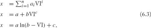
where VI is a combination (typically ratios) of reflectance values in n specific channels. The indices can be either computed using digital numbers, TOA radiance/reflectance, or surface radiance/reflectance.

A key issue to design VIs considers the characteristics of the soil reflectance. Let us illustrate how differences between the visible red and near-infrared (NIR) bands of a Landsat image can be used to identify areas containing significant vegetation. Figure 6.2 shows a standard color-infrared (CIR) composite of the image before and after a decorrelation stretching. This operation emphasizes spectral differences across the scene. Healthy, chlorophyll-rich vegetation has a high reflectance in the NIR (highlighted here in green). By looking at the differences between the NIR and the red channels, it is possible to quantify this contrast in spectral content between vegetated areas and other surfaces such as pavement, bare soil, buildings, or water. The Normalized Difference Vegetation Index (NDVI) [Liang, 2004, Rouse et al., 1973] is the most widely used index in the literature and is defined as:

Figure 6.2: Landsat image acquired over a residential area containing different land classes (asphalt, forest, buildings, grass, water, etc.). Left to right: standard color-infrared (CIR) composite, stretched CIR and NDVI image, thresholded NDVI image, and the scatter plot of all image pixels in Red versus NIR space.

The idea underlying this expression is that the difference between the NIR and the red should be large for high chlorophyll density (see Chapter 3). The normalization simply discounts the effects of uneven illumination, such as shadows of clouds or hills. A common practice to identify significant vegetation in an image consists on applying a simple threshold to the NDVI image, as shown in the fourth panel of Fig. 6.2.

A scatter plot of all image pixels in the space Red-NIR shows a clear positive linear correlation of the soil reflectances. The red line that limits the triangular-shaped distribution is called the soil line (in red in the rightmost panel of Fig. 6.2). It is also worth noting that those pixels with higher NIR reflectance and lower red reflectance are dense vegetation canopies. Over a vegetated surface, this line often constitutes the base of a triangle shape that is taken as a normalization factor of many VIs. In this optic, many corrected VIs such as the mSAVI (Improved Soil-Adjusted Vegetation index, [Qi et al., 1994]) and the TSAVI (Transformed Soil-Adjusted Vegetation Index, [Rondeaux et al., 1996]) have been proposed in the inversion literature.

Empirical approaches typically rely on carefully selected band ratios. Many indices focus on the red-edge reflectance, while others rely on describing the triangular-shaped distribution and on the area under the reflectance curve [Liang, 2008]. Section 6.5 shows a quantitative comparison of the most common indices for the particular case of estimating surface chlorophyll content from hyperspectral images. For a comprehensive revision of other indices, see [Liang, 2004, 2008]. Finally, we should note that indices are sensor-specific because of their particular spectral configurations. Figure 6.3[left] shows a vegetation index obtained with AVHRR.

Non-parametric methods

Several nonparametric approaches have been introduced for land parameter retrieval. In [R. and Nichol, 2011], biomass was estimated using common spectral band ratios, vegetation indices and linear/stepwise multiple regression models. Partial least squares (PLS) regression has been used for mapping canopy nitrogen [Coops et al., 2003, Townsend et al., 2003], analyzing biophysical properties of forests [Naesset et al., 2005], and retrieving leaf fuel moisture [Li et al., 2007]. PLS is a very popular method because it can cope with the existing high correlation between variables in a very efficient way.

The limitations of these regression tools have been circumvented by the introduction of nonlinear methods. Neural networks have been mainly used in combination of RTMs (we will come back to this hybrid approaches later). Nonlinear extension of PLS has been introduced via kernels in [Arenas-García and Camps-Valls, 2008]. Recently, the support vector regression (SVR) [Smola and Schölkopf, 2004] has yielded good results in modeling many biophysical parameters. In land applications, SVR is becoming a standard method that has proven high efficiency in modelling LAI [Durbha et al., 2007]. Several novel formulations of SVR have been recently presented, ranging from semisupervised methods (see Section 4.5.1) that exploit the wealth of unlabeled data in addition to the few labeled points [Bazi and Melgani, 2007, Camps-Valls et al., 2009], to multiouput SVR regression to provide estimations of several variables of interest simultaneously [Tuia et al., 2011b]. A review of SVR in remote sensing can be found in [Mountrakis et al., 2011].

In the recent years, the introduction of Gaussian Processes (GPs) [Rasmussen and Williams, 2006] techniques has alleviated some shortcomings of the previous methods. For instance, training GPs is far more simpler than neural networks. In addition, unlike in SVR, one can optimize very flexible kernels by maximum likelihood estimation. GPs generally yield very good numerical performance and stability. An application of GP to the estimation of land parameters can be found in [Furfaro et al., 2006]. Besides, GPs may be of particular interest because they do not only provide pointwise predictions but also confidence intervals for the predictions. A GP with a kernel adapted to both signal and noise properties was proposed for land parameter estimation in [Verrelst et al., 2011]. The method can provide a ranking of features (bands) and samples (spectra) for the task at hand. Section 6.5 gives empirical evidence of the GP advantages compared to other parametric and nonparametric methods.

6.2.2 OCEAN INVERSION MODELS

Open waters cover about three quarters of our planet’s surface [Campbell, 2007]. Monitoring the processes involved in oceans, rivers, lakes or ice and snow covers is of paramount relevance for both managing human settlements and controlling planet changes. In this context, the field is vast and many model inversion methods have been developed, mainly related to specific sensors or particular applications. This section briefly reviews the main contributions in hydrospheric sciences according to a series of application areas.

Figure 6.3: Sample products illustrating land, ocean and atmospheric products obtained by model inversion from satellite sensors. Left: AVHRR vegetation index over land and CZCS Ocean Colour phytoplankton concentration over sea in Europe and North Africa. Middle: Mediterranean sea-surface temperature from the Medspiration products. ESA’s Sentinel-3 mission for GMES will also provide data on sea-surface temperature. Right: Mean nitrogen dioxide (NO₂) pollution map for 2006, measured by Envisat’s Scanning Imaging Absorption Spectrometer for Atmospheric Chartography (SCIAMACHY) instrument, which records the spectrum of sunlight shining through the atmosphere. Source: ESA, http://www.esa.int

Parametric methods

In oceanic models, the particular characteristics of color or ocean salinity can be of interest [O’Reilly et al., 1998]. Between the 1970 and the 1990, Landsat images were introduced to inventory, locate and identify water. In Philipson and Hafker [1981], Landsat MSS images were used to identify flooded areas: a very simple ratio comparing the brightness in the near infrared (band 4) was implemented. Later, in [Frazier and Page, 2000], also included band 5 to identify turbid water and separate such areas from the unflooded land. It should be noted that several researchers have focused on detecting coastal or riverine floods (e.g., see http://floodobservatory.colorado.edu/). Another interesting issue is that of finding water in desert areas. Geologists have used remote sensing images to identify the new supplies of water in the rocks beneath the Sahara desert¹.

The sea surface salinity (SSS) parameter is one of the most relevant ones in ocean remote sensing [Lagerloef et al., 1995]. The flow intrusions with low salinity influence the deep thermohaline circulation, the meridional heat transport, and the near-surface dynamics of tropical oceans. Also, it has been argued that salinity is related to El Niño dynamics. The problems and limitations identified 15 years ago are still present. Nevertheless, the recent ESAâ^™s SMOS Mission [Kerr et al., 2001] has been launched to demonstrate the use of interferometry to observe salinity over oceans and ice characteristics, among other parameters. The main retrieval method uses a ratio-based parametrization of the measured brightness temperature of the Earth’s surface at horizontal and vertical polarizations [Font et al., 2004].

The estimation of the sea surface temperature (SST) plays a crucial role in many environmental models, such as those estimating energy and mass exchanges between atmosphere and surface, numerical weather prediction models or climatic variability and global ocean circulation models [Dash et al., 2002]. Many algorithms have been proposed for retrieving SST from space radiometry [Haines et al., 2007]. Most of them are derived from radiative transfer theory and require prior information about the state of the atmosphere (e.g., temperature and water vapor profiles) [Barton, 1992, Chan and Gao, 2005]. Figure 6.3[middle] shows an illustrative example of a sea-surface temperature map obtained from the Medspiration products².

Empirical ocean color algorithms for deriving chlorophyll concentrations have been developed primarily using spectral blue-to-green ratios and have been validated with field data collected from a number of stations. Garver and Siegel [1997] developed a nonlinear statistical method for the inversion of ocean color data, which assumed the known spectral shapes of specific absorption coefficients. The model was later improved in [Maritorena and O’Reilly, 2000, O’Reilly et al., 1998]. Lee et al. [2002] developed a multiband quasi-analytical model involving low computational cost and moderate accuracy. Recently, Shanmugam et al. [2011] introduced a new inversion model to retrieve the particulate backscattering in both coastal and ocean waters. The method is compared to a quasi-analytical algorithm (QAA), a constrained linear matrix inversion model (LM) with statistical selection, and the Garver-Siegel-Maritorena’s model. In Section 6.5, we also consider the problem of retrieval of oceanic chlorophyll concentrations.

Water quality assessment is another interesting application field for remote sensing parameter retrieval. In [Khorram, 1980], Landsat multispectral scanner (MSS) data, and U-2 colour and colour infrared photographs were combined with in-situ data for the assessment of water quality parameters: the water quality parameters of interest included turbidity and suspended solids. Later, in [Zhang and Chen, 2002], authors used a semi-empirical algorithm of water transparency with concurrent in situ measurements, Landsat TM and simulated SeaWiFS.

Finally, we should also mention the related fields of bathymetry and altimetry, where parametric models are extensively used. On the one hand, the field of bathymetry is concerned with the description of the water depth and ocean’s floor. Landsat MSS1 bands 4 and 5 have been used to define depth-finding algorithms [Polcyn and Lyzenga, 1979]. Other parametric models commonly used involve other MSS bands [Jupp et al., 1985]. Lyzenga et al. [1979] suggested logarithmic relations between depth zones and reflectance values, while polynomial regression was used in [Polcyn and Lyzenga, 1979]. On the other hand, in the field of altimetry, one measures sea surface slopes and currents. The main parameters involved in the model inversion are wave height, wind speed and sea levels. Most of the parameters have a seasonal behavior so, in the recent years, multitemporal images are jointly exploited to improve estimations. An interesting application of altimetry along with atmosphere modeling is the observation of hurricanes since both temperature and sea height are altered by its presence.

Non-parametric methods

Non-parametric and non-linear regression techniques have been effectively introduced for the estimation of ocean biophysical parameters. For example, neural networks have been considered for the estimation of chlorophyll concentration [Bruzzone and Melgani, 2005, Keiner, 1999], water quality [Cipollini et al., 2001] or ocean color in coastal waters [Camps-Valls and Bruzzone, 2009, Dzwonkowski and Yan, 2005]. SVR have been applied successfully for coastal chlorophyll concentration in [Bruzzone and Melgani, 2005, Camps-Valls et al., 2006a, Kwiatkowska and Fargion, 2003, Zhan, 2005]. Non-parametric Bayesian approaches have also been used for retrieval. The standard formulation of the Relevance Vector Machine (RVM) [Tipping, 2001] was modified in [Camps-Valls et al., 2006c] to incorporate prior knowledge in the iterative optimization procedure, and showed good performance for the estimation of ocean chlorophyll concentration. Finally, GP have also been considered for this task in [Pasolli et al., 2010].

6.2.3 ATMOSPHERE INVERSION MODELS

Atmospheric modeling involves estimation of pollution indicators, trace gases (such as ozone or metane), temperature and water vapor [Rodgers, 2000].

Parametric methods

With the introduction of meteorological satellites, the possibility to estimate temperature and moisture profiles became possible. Kapla [1959] studied parametric relations between the vertical distribution of temperature in the atmosphere and the measured thermal emission from the 15μm band of CO₂. Also, King [1956] estimated the temperature profile by measuring the angular distribution of emitted radiation in a single spectral interval. A detailed method for atmospheric remote sensing sounding from satellites appeared in [Wark, 1961, Yamamoto, 1961]. More recently, thanks to the launching of the first sounders, such as the Infrared Interferometer Spectrometer (IRIS) or the Satellite Infrared Spectrometer (SIRS), the field of model inversion developed quite rapidly. Current sounders like AIRS or IASI have demanded more studies in model inversion due to the challenges posed by the huge data volume acquired, which makes the ill-posed problem even harder.

There are many parametric methods available in the literature used for doing model inversion. The Bayesian approach to estimation basically involves including prior knowledge about the state vector X (e.g., the temperature profile) given the radiances y. By applying Bayes’ rule, a reasonable selection for the estimated state vector is the value of P(X|y) that has the highest probability, i.e., the maximum a posteriori (MAP) estimator. An alternative to MAP consists of the minimization of a loss function. The MSE is commonly adopted and results in the called Bayes Least Squares (BLS) [Blackwell, 2002]. This approach is inefficient because it requires assuming (or having access to) a complete representation of the relation between y and X, which is not typically available. This is why sometimes one constrains the estimator to be linear, thus leading to the linear least squares estimator (LS). However, in that case, only second order relations are taken into account.

The previous methods make use only of the statistical relations between state vectors and radiances. Other parametric approaches exploit the forward model as well. One example is the minimum information retrieval (MIR), which only depends on a nominal state X_o. An alternative to this method is the maximum-resolution retrieval (MRR), which assumes a forward model and a linear retrieval model. The method can inherit the classical problem of maximizing the resolution while simultaneously minimizing the noise [Blackwell, 2002]. This is why some regularized and constrained versions of MRR exist in the literature.

In the last decade, researchers have turned to the use of nonlinear methods such as neural networks or support vector machines for retrieval. These methods typically overcome many of the aforementioned problems. Figure 6.3[right] shows an illustrative example of the estimated mean map of nitrogen dioxide (NO₂) pollution from Envisat’s SCIAMACHY instrument³.

Non-parametric methods

Neural networks have been considered for the estimation of temperature and water vapor profiles using hyperspectral sounding data [Aires, 2002, Blackwell, 2005]. The classical multilayer perceptron was chosen in both cases. In [Camps-Valls et al., 2011], results of standard multilayer neural networks, cascade neural nets and least squares SVM are given for the estimation of temperature and moisture profiles (see Section 6.5). NO₂ emissions from biomass burning was estimated in [Bruzzone et al., 2003], while the challenging problem of hourly surface ozone concentrations was successfully addressed with different topologies of dynamic neural networks in [Balaguer-Ballester et al., 2002]. SVR have also been considered for extracting atmospheric properties [Camps-Valls et al., 2011] or continental evapotranspiration processes [Yang et al., 2006]. In [Xie et al., 2008], SVR was used to estimate horizontal water vapor transport from multisensor data.

6.3 PHYSICAL INVERSION TECHNIQUES

The previous statistical approaches may lack transferability, generality, or robustness to new geographical areas. This has led to the advancement of physical models for estimating bio-geo-chemical structural state variables from spectra. The advantage of physical models is that they can be coupled from lower to higher levels (e.g., canopy level models build upon leaf models), thereby providing a physically-based linkage between optical EO data and biochemical or structural state variables [Jacquemoud et al., 2009, Verhoef and Bach, 2003]. RTMs can be applied in many ways for forestry applications; some can be run in the forward mode, while others in both forward and inverse modes:

The basic assumption for inverting RTMs is that the forward model contains all the necessary information about the problem, so its inversion may lead to accurate parameter estimates. There exist many RTMs implemented in software packages to deal with the forward modeling. For example, PROSPECT is an RTM accounting for leaf optical properties [Jacquemoud and Baret, 1990] while SAIL constitutes a canopy bidirectional reflectance model [Verhoef, 1984]. Their combination led to the PROSAIL model: advances on joint strategies are revised in [Jacquemoud et al., 2009]. While PROSPECT and SAIL are RTMs more focused on land/vegetation quantitative problems, other RTMs are more specific to ocean or atmosphere applications. For example, the optimal spectral sampling (OSS) is a fast and accurate monochromatic RTM well-suited for geophysical parameter retrieval [Moncet et al., 2008].

The design of accurate forward models is subject of active research [Asrar, 1989, Goel, 1989, Kimes et al., 2000, Liang, 2004, Pinty and Verstraete, 1991]. In this chapter, however, rather than reviewing the physical aspects of RTMs, we will focus on the different families of inversion methodologies, their assumptions, advantages and shortcomings, along with the common applications. Several inversion approaches have been considered in the literature [Baret and Buis, 2008, Liang, 2004, 2008]: classical iterative optimization, look-up-tables (LUTs), simulated annealing and genetic algorithms [Fang and Liang, 2003, Renders and Flasse, 1996], Markov chain Monte Carlo (MCMC) [Zhang et al., 2005b], and alternative Bayesian approaches. Nevertheless, iterative optimization and (or over) LUTs are the most widely used [Liang, 2008].

6.3.1 OPTIMIZATION INVERSION METHODS

Optimization methods tackle the inverse problem in Eq. (6.1) by minimizing a loss function, (θ), respect to the state parameters, θ. To do this, a set of n data pairs generated by a particular RTM, are used. Different norms of the residuals can be used here. Some authors assume a Gaussian model for the uncertainties (residuals), thus minimizing the ₂-norm, min_θ{||y − f(X; θ)||²}. Nevertheless, the most important issue is the inclusion of prior knowledge in the minimization functional accounting for model uncertainties, and several norms have been used in this sense [Bacour et al., 2002]. Other authors impose sparsity constraints or the (reasonable) positivity of the retrievals. The goal of these approaches is not only to obtain more realistic estimates but improving the convexity of the error surface [Combal, 2002].

In most of the cases, however, the most accurate physically-based models are non-differentiable and involve computationally expensive inversion methods. Classical techniques include: simplex methods, which are particularly useful for discontinuous, noisy or numerically-deficient functions; the (iterative) conjugate direction set method [Press et al., 1989], which may be suitable when many parameters are involved in the inversion; or adjoint models that provide (approximate) analytical expressions for the loss gradient (see [Liang, 2008] and references therein). In any case, the main problems of optimization inversion methods are typically related to the high computational cost involved, and the risk of falling into local minima. While the latter has been recently alleviated [Bonnans et al., 2006], the former constitutes a serious drawback for the adoption in operational regional or global studies.

Despite all these disadvantages, these methods are widely used in gneral. A good review on optimization methods used in remote sensing for land applications can be found in [Bacour et al., 2002]. Their main advantage is the flexibility and the easy inclusion of prior knowledge, while the main applications involve estimating vegetation parameters. For example, numerical inversion on POLarization and Directionality of the Earth’s Reflectances (POLDER)⁴ data was presented in Bicheron and Leroy [1999] for retrieving both LAI and fraction of photosynthetically active radiation (FPAR), while several canopy reflectance models were compared in [Jacquemoud et al., 2000] to estimate chlorophyll content, the leaf area index, and the mean leaf inclination angle. Later, in [Zarco-Tejada et al., 2001], hyperspectral data was used for chlorophyll content estimation using a numerical model inversion approach coupled to the PROSPECT model. Houborg et al. [2007] retrieved LAI, chlorophyll content, and total vegetation water content using Terra and Aqua MODIS multi-spectral, multi-temporal, and multi-angle reflectance observations. In Gemmell et al. [2002], boreal forest cover and tree crown transparency was obtained from Landsat TM data. In this case, inclusion of ancillary data became necessary to regularize the solution.

6.3.2 GENETIC ALGORITHMS

The main problems faced in the previous optimization approaches are the convergence to an optimal solution, the dependence on the initialization parameters of the algorithms, and the associated high computational cost. Genetic algorithms [Goldberg, 1989] can be an alternative solution. Unfortunately, very few contributions are found in the literature so far: retrieval of land surface roughness and soil moisture [Wang and Jin, 2000], forest parametrization [Lin and Sarabandi, 1999], LAI estimation from either optical [Fang and Liang, 2003] or thermal infrared multiangle data [Zhuang and Xu, 2000]. In [Lin and Sarabandi, 1999], GA are used for the retrieval of forest parameters using a fractal-based coherent scattering model. Also water optical properties have been derived [Slade et al., 2004, Zhan et al., 2003].

6.3.3 LOOK-UP TABLES

This approach considers constructing a database, or Look-up table (LUT), of representative spectra and associated state parameters. For every new incoming spectra, a simple criterion of search can be applied to assign the most appropriate parameter. The advantages are clear: building the LUT is an off-line process so computationally cheap, the minimization criterion (typically based on RMSE) is simple to apply and leads to a global solution. Behind this theoretical simplicity, important problems arise [Weiss et al., 2000]. First, building a representative LUT that accounts for most of uncertainties and properly covers the parameter space is a difficult task [Combal, 2002, Weiss et al., 2000]. These problems give rise to very big LUTs, that are hardly manageable which, in turn, inducing slow searches. Second, the approach typically relies on heuristic criteria for both selecting the most representative cases (pairs of spectra and associated parameters) [Combal, 2002, Weiss et al., 2000], and the search criterion [Knyazikhin, 1998a, Knyazikhin et al., 1998].

Mainly due to its efficiency, the approach is widely adopted in prospective studies and in operational product generation, such as for retrieving LAI and FPAR products from surface reflectances in the Moderate Resolution Imaging Spectroradiometer (MODIS)⁵ and the Multiangle Imaging SpectroRadiometer (MISR)⁶ [Knyazikhin, 1999, Myneni et al., 2002]. Darvishzadeh et al. [2008] obtained LAI and leaf and canopy chlorophyll contents by inverting the PROSAIL model. This is a very popular approach, mainly for works addressing a single test site (e.g., with airborne data). In [González-Sanpedro et al., 2008], LAI was derived from a multitemporal series of images inverting the PROSPECT+SAIL model. In this case, the LUT was designed to take into account the different crop types present in the area.

6.3.4 BAYESIAN METHODS

Model inversion following Bayesian approaches try to approximate the posterior distribution, p(X|y), i.e., the distribution of the variables given the reflectance/radiance. The main advantages rely on the fact that no assumption about data distributions need to be done. Nevertheless, the approach has been scarcely adopted, mainly due to high computational cost of iterative approaches such as the Markov chain Monte Carlo (MCMC) [Zhang et al., 2005b]. The alternative Importance Sampling (IS) [Makowski et al., 2006] alleviates this problem but has not been extensively evaluated in remote sensing applications. A Bayesian estimation for land surface temperature retrieval was presented in [Morgan, 2005], and for soil moisture retrieval in [Notarnicola et al., 2008].

6.4 HYBRID INVERSION METHODS

In recent years, combined approaches that use the databases generated by RTMs and powerful regression approaches have been introduced in the literature. These hybrid methods try to exploit the advantages of physically-based models and the flexibility and computational efficiency of nonparametric nonlinear regression methods. The idea is to learn the inverse mapping g of Eq. (6.2) with, for example, neural networks using data generated by accurate RTMs. Several nonparametric methods have been applied to invert RTMs, from decision trees to neural networks and kernel methods. The main issue is how representative is the dataset because inversion will not be possible (or deficient) if the parameter space is poorly sampled. This poses several related problems: how many data points are necessary for representing the problem, how many input (parameters) and output (spectra) dimensions should enter the RTM, and how should one train regression methods in such potentially complex situations. Several families of methods have been used so far, which are briefly summarized below.

6.4.1 REGRESSION TREES

Regression trees have been used to estimate land surface variables: Weiss and Baret [19991] retrieved LAI, fraction of photo-synthetically active radiation (FAPAR) and chlorophyll content from VEGETATION/SPOT4⁷; Gong et al. [1999] inverted LAI from a simulated database; Fang et al. [2003] inverted LAI from the Landsat ETM imagery⁸; Liang et al. [2003] estimated LAI and broadband albedo from the Earth Observing 1 (EO-1)⁹ data by incorporating the soil line concept; Kimes et al. [2002] inverted a complex 3D DART model for a wide range of simulated forest canopies using POLDER-like data; and broadband land surface albedo was estimated in [Liang et al., 2003].

6.4.2 NEURAL NETWORKS

The vast majority of hybrid inversion methods consider the use of neural networks [Baret and Fourty, 1997, Baret et al., 1995, Gopal and Woodcock, 1996, Jin and Liu, 1997, Kimes et al., 1998, Smith, 1993] for retrieval of canopy parameters. Actually, with the current neural network implementations, they are fast to train a test. Vasudevan et al. [2004] used neural nets for deriving integrated water vapor and cloud liquid water contents over oceans from brightness temperatures measured by the Multifrequency Scanning Microwave Radiometer (MSMR). Fang and Liang [2005] noted deficiencies in LAI retrieval by standard LUT methods, and compared neural nets and projection pursuit to obtain less biased estimates. In [Bacour et al., 2006], the network was trained on a reflectance database made of RTM simulations, and LAI, FAPAR and FCOVER were accurately retrieved as compared with ground measurements. Very recently, the combination of clustering and neural networks inverted simulated data with additive noise. Inclusion of multiangle images improved the LAI estimations. Lately, in [Verger et al., 2011], neural networks were successfully developed over RTMs to estimate LAI, FCOVER and FAPAR.

6.4.3 KERNEL METHODS

Only very recently, the use of kernel methods [Camps-Valls and Bruzzone, 2009], such as the support vector regression (SVR) or the kernel ridge regression (KRR) have been used. In [Durbha et al., 2007], LAI is retrieved by inverting PROSAIL using SVR over Multi-angle Imaging SpectroRadiometer (MISR) data¹⁰. In our recent work [Camps-Valls et al., 2011], linear regression, multilayer perceptrons, cascade neural nets and kernel ridge regression were used to invert the OSS transfer model for atmospheric parameter retrieval. The advantage of the approach allowed improved accuracy versus standard optimal estimation approaches¹¹, and great computational savings for inversion and retrieval.

6.5 EXPERIMENTS

This section illustrates the application of the three inversion approaches revised (statistical, physical and hybrid) in land, ocean and atmospheric parameter retrieval applications.

6.5.1 LAND SURFACE BIOPHYSICAL PARAMETER ESTIMATION

The first application deals with the statistical approach to retrieve vegetation parameters using in situ measurements and hyperspectral images. We compare the most representative parametric approaches, and state-of-the-art nonparametric methods, such as SVR [Smola and Schölkopf, 2004], GP [Rasmussen and Williams, 2006, Verrelst et al., 2011] and the recently presented multi-output SVR (MSVR) [Tuia et al., 2011b].

The data were obtained in the SPARC-2003 (SPectra bARrax Campaign) and SPARC-2004 campaigns in Barrax, La Mancha, Spain. The region consists of approximately 65% dry land and 35% irrigated land. The methodology applied to obtain the in situ leaf-level Chl_ab data consisted of measuring samples with a calibrated CCM-200 Chlorophyll Content Meter in the field. Concurrently, we used CHRIS images Mode 1 (62 spectral bands, 34m spatial resolution at nadir). The images were preprocessed [Gómez-Chova et al., 2008], geometrically [Alonso and Moreno, 2005] and atmospherically corrected [Guanter et al., 2005]. Summarizing, a total of n = 136 datapoints in a 62-dimensional space and the measured chlorophyll concentration constitute the database.

Performances of a wide array of established indices, linear regression with all bands, SVR, MSVR and GP were tested. Models were run for a total of 50 random realizations of the training and test data. Averaged correlation coefficients are shown for the test set in Table 6.1. It is clearly observed that nonparametric methods show the best results in both correlation and stability, with GP performing best of the tested methods.

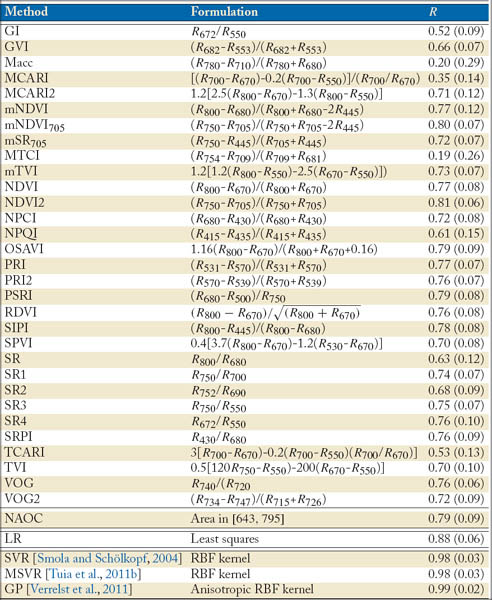
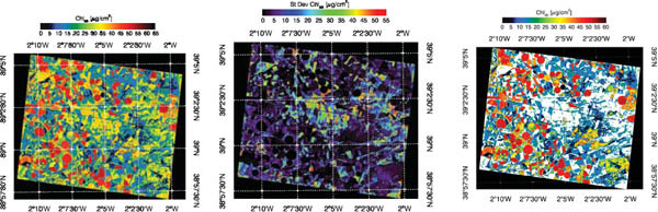
Figure 6.4: Final chlorophyll concentration prediction map (left) and predictive standard deviation (middle) and masked confidence map (right) generated with GP on the CHRIS 12-07-2003 nadir image.

The best GP model was used for prediction on the whole CHRIS image to generate a pixel-by-pixel map of Chl and its confidence map (see Fig. 6.4). The maps show clearly the irrigated crops (the circles in orange-red), the semi-natural areas (light blue) and the bare soil areas (dark blue). Although these maps cannot be used as a validation per se, the confidence maps allow us to draw conclusions on the performance of the retrievals. For example, the high confidences (western part of the image) were the fields sampled the most, while low confidence predictions (center of the image) correspond to areas particularly underrepresented in the training data, such as dry barley, harvested barley, and bright bare soils. This product may be used to set sensitivity margins of field instruments quite intuitively: areas are thresholded with error levels above 10% of the total Chl range (e.g., >6.5μg/cm⁻²), see Fig. 6.4[right]. These results confirm the very good properties of nonparametric models in general and GPs in particular for the estimation of land cover properties from space, applicable for both multispectral and hyperspectral sensors.

6.5.2 OPTICAL OCEANIC PARAMETER ESTIMATION

In this section, performance of neural networks, SVR, RVM and GP in the estimation of oceanic chlorophyll concentration from measured reflectances is compared in terms of accuracy, bias, and sparsity. The SeaBAM dataset is used [O’Reilly et al., 1998], which gathers 919 in-situ measurements of chlorophyll concentration around the United States and Europe. The dataset contains in situ pigments and remote sensing reflectance measurements at wavelengths present in the SeaWiFS sensor.¹²

Table 6.2 presents results in the test set for all models. For comparison purposes, we include results obtained with a feedforward neural network trained with back-propagation (NN-BP), which is a standard approach in biophysical parameters retrieval. Also, we include results for standard parametric models (Morel, CalCOFI and OC families) [Maritorena and O’Reilly, 2000]. We can observe that (1) SVR, RVM and GP show a better performance than empirical Morel and OC2 models, and also better than artificial neural networks (NN-BP); (2) the SVR and GP techniques are more accurate (RMSE, MAE); (3) RVM and GP are less biased (ME) than the rest of the models; and (4) in the case of the RVMs, drastically much more sparse (only 4.9% of training samples were necessary to attain good generalization capabilities). Comparing SVR and RVM, we can state that RVMs provide accurate estimations (similar to SVR) with small number of relevant vectors. Nevertheless, GPs provide more accurate results than SVR and RVM.

These results suggest that GPs are potentially useful methods for ocean chlorophyll concentration estimation. We did a one-way analysis of variance (ANOVA) to compare the means of the models and no significant statistical differences were observed between the nonparametric approaches for accuracy (p = 0.31) and bias (p = 0.33). Therefore, as a preliminary conclusion, we can state that the nonparametric solutions are more accurate than parametric or physical models.

Figure 6.5 shows a comparison between the predictions obtained by the GP model and the OC4 model. In the same figure, we also show the predicted values against the residuals for these models. These goodness-of-fit graphics confirm the good predictive performance of both models. However, some differences can be observed. Excellent coefficient of determination (R² = 0.955, test set) and unbiased estimations (Slope: 1.001±0.010, intercept: 0.001±3e-9) and errors are observed for the RVM, which are slightly better than those shown by the OC4 model (R² = 0.933, Slope: 1.088±0.034, intercept: 0.055±3e-5). In particular, it is worth to note the much higher bias in the prediction errors versus residuals obtained by the OC4 (compare fitted regression lines in Fig. 6.5(b) and (d)). This is an important second characteristic of the model since unbiased estimations are desirable in estimating biophysical parameter, see the mean error in Table 6.2.

Figure 6.5: Performance of the OC4 (a,b) and GP (c,d) in the test set. Predicted versus observed concentrations, and predicted versus residuals are depicted.

6.5.3 MODEL INVERSION OF ATMOSPHERIC SOUNDING DATA

Temperature and water vapor are atmospheric parameters of high importance for weather forecast and atmospheric chemistry studies [Hilton et al., 2009, Liou, 2002]. Nowadays, observations from spaceborne high spectral resolution infrared sounding instruments can be used to calculate the profiles of such atmospheric parameters with unprecedented accuracy and vertical resolution [Huang et al., 1992]. In this section we use data acquired by the Infrared Atmospheric Sounding Interferometer (IASI) [Siméoni et al., 1997] (see Chapter 2 for details).

This section presents results on the use of linear regression (LR), multilayer neural networks (NN), cascade neural networks (CNN), and kernel ridge regression (KRR) to derive temperature and moisture profiles from hyperspectral infrared sounding spectra [Camps-Valls et al., 2011]. We followed an hybrid approach: first we generated data using an RTM and then trained the nonparametric regression models. Test results are shown on a full IASI orbit (91800 IFOVs in 2008-03-04). As ancillary data we used AVHRR data, which has a much finer spatial resolution and thus allows proper visual inspection and comparison of the results. A total amount of 67475 synthetic FOVs were simulated by the European Organisation for the Exploitation of Meteorological Satellites (EUMETSAT)¹³ with the OSS infrared radiative transfer code [Moncet et al., 2008] according to input profiles of temperature and humidity given in 90 pressure levels. The state vector (output space) to be retrieved consists of temperature and water vapor profiles. The range between [100, 1000] hPa is sampled at 90 pressure levels, thus constituting a challenging nonlinear multi-output regression problem.

A total of 4699 channels were retained by removing noisy channels [Calbet and Schlüssel, 2005]. Then, PCA was performed and the optimal number of components selected by training LR and KRR with standard cross-validation. The best results are shown in Fig. 6.6. The optimal linear combination of models in terms of MSE is also given. All nonlinear models outperform LR. Neural nets and KRR perform similarly, and, in general, no numerical differences (both in terms of RMSE and bias) are observed, while the OLC method reports an important gain for temperature estimation, yielding an average gain in RMSE of +0.6K. Model combination not only gives smoother error profiles (RMSE<1K) but also lower biases (ME<0.5K).

Figure 6.6: RMSE (solid) and bias (dashed) quality measures obtained with linear and nonlinear regression for the case of real MetOp-IASI data in cloud-free and emissivity ‘sea’ scenarios. The number of used features after PCA is indicated in the legend for each regression method.

Figure 6.7 illustrates the results obtained by KRR in some areas of interest. For the case of Madagascar, it is clear that big errors in temperature estimation, ΔT, highly correlate with the presence of clouds. Low confidence values are assigned to cloudy regions, see e.g., north-east Madagascar and south-west Mexico images.

6.6 SUMMARY

This chapter revised one of the most active fields in remote sensing image processing: the estimation of physical parameters from acquired images and in-situ measurements. We presented the main approaches in the literature and introduced the principles and standard terminology. A thorough comparison between all approaches is still missing in the literature but it seems that hybrid methods embracing physics and statistics provide accurate and computationally efficient methods. Several real application examples were provided in land, ocean and atmospheric parameter retrieval, and confirmed the excellent results obtained by nonparametric statistical approaches, either alone or in combination with radiative transfer models. The future poses some challenging problems: just to name a few, we will be confronted to the availability of huge amount of training data, to the design of more sophisticated and realistic RTMs, to the combination of both statistical and physically-based models, and to the specification of models that can adapt to multitemporal domains.

Figure 6.7: Illustrative examples of prediction errors for Madagascar [top] and Mexico [bottom]. We show the AVHRR radiance in channel 4 for visual inspection, the discrepancies of KRR predictions with the ECMWF ground truth, and the KRR predictive variance (in log-scale for proper visualization), which was computed as in GPs.

¹http://www.nae.edu/File.aspx?id=7423

²http://projets.ifremer.fr/cersat/Information/Projects/
MEDSPIRATION2

³http://envisat.esa.int/instruments/sciamachy/

⁴http://smsc.cnes.fr/POLDER/

⁵http://modis.gsfc.nasa.gov/

⁶http://www-misr.jpl.nasa.gov/

⁷http://www.spot-vegetation.com/

⁸http://landsat.gsfc.nasa.gov/

⁹http://eo1.gsfc.nasa.gov/

¹⁰http://www-misr.jpl.nasa.gov/

¹¹Optimalestimation (OE) refers to a collection of inversion techniques for deriving physical properties from satellite measurements. The methods have relatively high accuracy and can incorporate prior knowledge. However, OE is a very computationally demanding method because, in general, the forward model has to be called iteratively several times for each pixel. Even for fast RTMs, like the OSS used here, this involves obtaining predictions in hours or even days. We address the reader to [Rodgers, 2000] for an excellent book on inverse methods for atmospheric sounding, including details on the optimal estimation theory.

¹²More information at http://seabass.gsfc.nasa.gov/seabam/seabam.html.

¹³www.eumetsat.int/