
Chapter 10. Operations
- Monitoring and metrics
- Performance testing and tuning
- Common management and operations tasks
- Backup and replication strategies
You’ve covered a lot of ground in understanding HBase and how to build applications effectively. We also looked at how to deploy HBase clusters in a fully distributed fashion, what kind of hardware to choose, the various distribution options, and how to configure the cluster. All this information is useful in enabling you to take your application and HBase into production. But there is one last piece of the puzzle left to be covered—operations. As a developer of the application, you wouldn’t be expected to operate the underlying HBase cluster when everything is in production and the machines are churning full speed. But in the initial part of your project’s HBase adoption, chances are that you’ll be playing an integral role in the operations and helping the ops team get up to speed with all the aspects of operating an HBase cluster in production successfully.
Operations is a broad topic. Our goal for this chapter is to touch on the basic operational concepts pertaining to HBase. This will enable you to successfully operate your cluster and have your application serve the end users that it was built to serve. To do this, we’ll start with covering the concepts of monitoring and metrics as they pertain to HBase. This will consist of the different ways you can monitor your HBase deployment and the metrics you need to monitor.
Monitoring is an important step, and once you have that in place, you’ll be in a good place to start thinking about performance testing your HBase cluster and your application. There’s no point making all that effort and taking a system to production if it can’t sustain the load of all the users who want to use it!
We’ll then cover common management and operations tasks that you’ll need during the course of operating a cluster. These include things like starting and stopping services, upgrades, and detecting and fixing inconsistencies. The last topic in the chapter pertains to backup and replication of HBase clusters. This is important for business-continuity purposes when disaster strikes.
Note
This chapter covers topics that are relevant to the 0.92 release. Some of the recommendations may change with future releases, and we encourage you to look into those if you’re using a later release.
Without further ado, let’s jump right in.
10.1. Monitoring your cluster
A critical aspect of any production system is the ability of its operators to monitor its state and behavior. When issues happen, the last thing an operator wants to do is to sift through GBs and TBs of logs to make sense of the state of the system and the root cause of the issue. Not many people are champions at reading thousands of log lines across multiple servers to make sense of what’s going on. That’s where recording detailed metrics comes into play. Many things are happening in a production-quality database like HBase, and each of them can be measured in different ways. These measurements are exposed by the system and can be captured by external frameworks that are designed to record them and make them available to operators in a consumable fashion.
Note
Operations is particularly hard in distributed systems because many more components are involved, in terms of both the different pieces that make up the system and the scale at which they operate.
Collecting and graphing metrics isn’t unique to HBase and can be found in any successful system, large or small scale. The way different systems implement this may differ, though. In this section, we’ll talk about how HBase exposes metrics and the frameworks that are available to you to capture these metrics and use them to make sense of how your cluster is performing. We’ll also talk about the metrics HBase exposes, what they mean, and how you can use them to alert you about issues when they happen.
Tip
We recommend that you set up your full metrics collection, graphing, and monitoring stack even in the prototyping stage of your HBase adoption. This will enable you to become familiar with the various aspects of operating HBase and will make the transition to production much smoother. Plus, it’s fun to see pretty graphs showing requests hitting the system when they do. It will also help you in the process of building your application because you’ll know more about what’s going on in the underlying system when your application interacts with it.
10.1.1. How HBase exposes metrics
The metrics framework is another of the many ways that HBase depends on Hadoop. HBase is tightly integrated with Hadoop and uses Hadoop’s underlying metrics framework to expose its metrics. At the time of writing this manuscript, HBase was still using the metrics framework v1.[1] Efforts are underway to have HBase use the latest and greatest,[2] but that hasn’t been implemented yet.
1 Hadoop metrics framework v1, Apache Software Foundation, http://mng.bz/J92f.
2 Hadoop metrics framework v2, Apache Software Foundation, http://mng.bz/aOEI.
It isn’t necessary to delve deeply into how the metrics frameworks are implemented unless you want to get involved in the development of these frameworks. If that’s your intention, by all means dive right into the code. If you’re just interested in getting metrics out of HBase that you can use for your application, all you need to know is how to configure the framework and the ways it will expose the metrics, which we’ll talk about next.
The metrics framework works by outputting metrics based on a context implementation that implements the MetricsContext interface. A couple of implementations come out of the box that you can use: Ganglia context and File context. In addition to these contexts, HBase also exposes metrics using Java Management Extensions (JMX).[3]
3 Qusay H. Mahmoud, “Getting Started with Java Management Extensions (JMX): Developing Management and Monitoring Solutions,” Oracle Sun Developer Network, January 6, 2004, http://mng.bz/619L.
10.1.2. Collecting and graphing the metrics
Metrics solutions involve two aspects: collection and graphing. Typically these are both built into the same framework, but that’s not a requirement. Collection frameworks collect the metrics being generated by the system that is being monitored and store them efficiently so they can be used later. These frameworks also do things like roll-ups on a daily, monthly, or yearly basis. For the most part, granular metrics that are a year old aren’t as useful as a yearly summary of the same metrics.
Graphing tools use the data captured and stored by collection frameworks and make it easily consumable for the end user in the form of graphs and pretty pictures. These graphs are what the operator looks at to quickly get insight into the status of the system. Add to these graphs things like thresholds, and you can easily find out if the system isn’t performing in the expected range of operation. And based on these, you can take actions to prevent the end application from being impacted when Murphy strikes.[4]
4 You’ve certainly heard of Murphy’s law: http://en.wikipedia.org/wiki/Murphy’s_law.
Numerous collection and graphing tools are available. But not all of them are tightly integrated with how Hadoop and HBase expose metrics. You’re limited to Ganglia (which has native support from the Hadoop metrics framework) or to frameworks that can collect metrics via JMX.
Ganglia
Ganglia (http://ganglia.sourceforge.net/)[5] is a distributed monitoring framework designed to monitor clusters. It was developed at UC Berkeley and open-sourced. The Hadoop and HBase communities have been using it as the de facto solution to monitor clusters.
5Monitoring with Ganglia, by Matt Massie et al., is expected to release in November 2012 and will be a handy resource for all things monitoring and Ganglia. See http://mng.bz/Pzw8.
To configure HBase to output metrics to Ganglia, you have to set the parameters in the hadoop-metrics.properties file, which resides in the $HBASE_HOME/conf/ directory. The context you’ll configure depends on the version of Ganglia you choose to use. For versions older than 3.1, the GangliaContext should be used. For 3.1 and newer, GangliaContext31 should be used. The hadoop-metrics.properties file configured for Ganglia 3.1 or later looks like the following:
hbase.class=org.apache.hadoop.metrics.ganglia.GangliaContext31
hbase.period=10
hbase.servers=GMETADHOST_IP:PORT
jvm.class=org.apache.hadoop.metrics.ganglia. GangliaContext31
jvm.period=10
jvm.servers= GMETADHOST_IP:PORT
rpc.class=org.apache.hadoop.metrics.ganglia. GangliaContext31
rpc.period=10
rpc.servers= GMETADHOST_IP:PORT
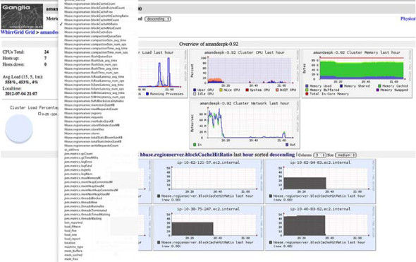
Once you have Ganglia set up and the HBase daemons started with these configuration properties, the metrics list in Ganglia will show metrics being spewed out by HBase, as shown in figure 10.1.
Figure 10.1. Ganglia, set up to take metrics from HBase. Notice the list of HBase and JVM metrics in the drop-down Metrics list.
JMX
Apart from exposing metrics using the Hadoop metrics framework, HBase also exposes metrics via JMX. Several open source tools such as Cacti and OpenTSDB can be used to collect metrics via JMX. JMX metrics can also be viewed as JSON from the Master and RegionServer web UI:
- JMX metrics from the Master: http://master_ip_address:port/jmx
- JMX metrics from a particular RegionServer: http://region_server_ip_address:port/jmx
The default port for the Master is 60010 and for the RegionServer is 60030.
File Based
HBase can also be configured to output metrics into a flat file. Every time a metric is to be output, it’s appended to that file. This can be done with or without timestamps, depending on the context. File-based metrics aren’t a useful way of recording metrics because they’re hard to consume thereafter. Although we haven’t come across any production system where metrics are recorded into files for active monitoring purposes, it’s still an option for recording metrics for later analysis:
To enable metrics logging to files, the hadoop-metrics.properties file looks like this:
hbase.class=org.apache.hadoop.hbase.metrics.file.TimeStampingFileContext
hbase.period=10
hbase.fileName=/tmp/metrics_hbase.log
jvm.class=org.apache.hadoop.hbase.metrics.file.TimeStampingFileContext
jvm.period=10
jvm.fileName=/tmp/metrics_jvm.log
rpc.class=org.apache.hadoop.hbase.metrics.file.TimeStampingFileContext
rpc.period=10
rpc.fileName=/tmp/metrics_rpc.log
Let’s look at the metrics that HBase exposes that you can use to get insights into the health and performance of your cluster.
10.1.3. The metrics HBase exposes
The Master and RegionServers expose metrics. You don’t need to look at the HBase code to understand these, but if you’re curious and want to learn about how they’re reported and the inner workings of the metrics framework, we encourage you to browse through the code. Getting your hands dirty with the code never hurts.
The metrics of interest depend on the workload the cluster is sustaining, and we’ll categorize them accordingly. First we’ll cover the general metrics that are relevant regardless of the workload, and then we’ll look at metrics that are relevant to writes and reads independently.
General Metrics
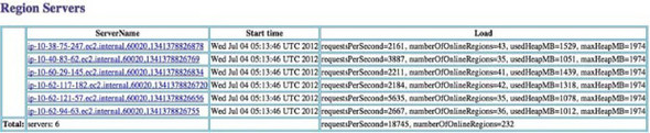
Metrics related to the system load, network statistics, RPCs, alive regions, JVM heap, and JVM threads are of interest regardless of the kind of workload being run; they can be used to explain the system’s behavior. The Master UI shows the heap usage and the requests per second being served by the RegionServers (figure 10.2).
Figure 10.2. The HBase Master web UI shows the number of requests per second being served by each of the RegionServers, the number of regions that are online on the RegionServers, and the used and max heap. This is a useful place to start when you’re trying to find out the state of the system. Often, you can find issues here when RegionServers have fallen over, aren’t balanced in terms of the regions and requests they’re serving, or are misconfigured to use less heap than you had planned to give them.
HBase metrics are important, but so are the metrics from dependency systems—HDFS, underlying OS, hardware, and the network. Often the root cause for behavior that is out of the normal range lies in the way the underlying systems are functioning. Issues there typically result in a cascading effect on the rest of the stack and end up impacting the client. The client either doesn’t perform properly or fails due to unexpected behavior. This is even more pronounced in distributed systems that have more components that can fail and more dependencies. Covering detailed metrics and monitoring for all dependencies is beyond the scope of this book, but plenty of resources exist that you can use to study those.[6]
6Hadoop Operations, by Eric Sammer, is a good resource for all things related to operating Hadoop in production. It’s expected to release in fall 2012. See http://mng.bz/iO24.
The important bits that you absolutely need to monitor are as follows:
- HDFS throughput and latency
- HDFS usage
- Underlying disk throughput
- Network throughput and latency from each node
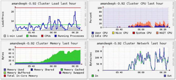
System- and network-level information can be seen from Ganglia (figure 10.3) and from several Linux tools such as lsof, top, iostat, netstat, and so on. These are handy tools to learn if you’re administering HBase.
Figure 10.3. Ganglia graphs showing a summary of the entire cluster for load, CPU, memory, and network metrics
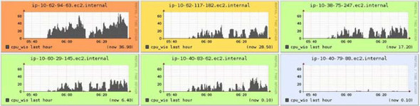
One interesting metric to keep an eye on is the CPU I/O wait percentage. This indicates the amount of time the CPU spends waiting for disk I/O and is a good indicator of whether your system is I/O bound. If it is I/O bound, you need more disks in almost all cases. Ganglia graphs for CPU I/O wait percentage from a cluster running a heavy write workload are shown in figure 10.4. This metric is useful when the read I/O is high as well.
Figure 10.4. CPU I/O wait percentage is a useful metric to use to understand whether your system is I/O bound. These Ganglia graphs show significant I/O load on five out of the six boxes. This was during a heavy write workload. More disks on the boxes would speed up the writes by distributing the load.
We’ve talked about some of the generic metrics that are of interest in a running cluster. We’ll now go into write- and read-specific metrics.
Write-Related Metrics
To understand the system state during writes, the metrics of interest are the ones that are collected as data is written into the system. This translates into metrics related to MemStore, flushes, compactions, garbage collection, and HDFS I/O.
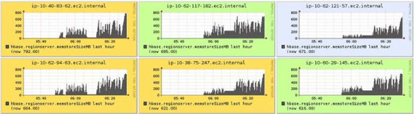
During writes, the ideal MemStore metrics graph should look like saw teeth. That indicates smooth flushing of the MemStore and predictable garbage collection overhead. Figure 10.5 shows the MemStore size metrics from Ganglia during heavy writes.
Figure 10.5. MemStore size metrics from Ganglia. This isn’t an ideal graph: it indicates that tuning garbage collection and other HBase configs might help improve performance.
To understand HDFS write latencies, the fsWriteLatency and fsSyncLatency metrics are useful. The write-latency metric includes the latency while writing HFiles as well as the WAL. The sync-latency metrics are only for the WALs.
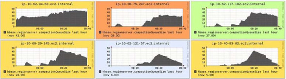
Write latencies going up typically also causes the compaction queues to increase (figure 10.6).
Figure 10.6. The compaction queues going up during heavy writes. Notice that the queue is higher in some boxes than the others. This likely indicates that the write load on those RegionServers is higher than on the others.
Garbage-collection metrics are exposed by the JVM through the metric context; you can find them in Ganglia as jvm.metrics.gc*. Another useful way of finding out what’s going on with garbage collection is to enable garbage-collection logging by putting the -Xloggc:/my/logs/directory/hbase-regionserver-gc.log flag in the Java options (in hbase-env.sh) for the RegionServers. This is useful information when dealing with unresponsive RegionServer processes during heavy writes. A common cause for that is long garbage-collection pauses, which typically means garbage collection isn’t tuned properly.
Read-Related Metrics
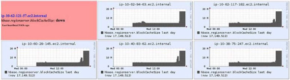
Reads are different than writes, and so are the metrics you should monitor to understand them. During reads, the metrics of interest relate to the block cache primarily, apart from the general metrics that we covered initially. The block-cache metrics for cache hits, evictions, and cache size are useful in understanding the read performance; you can tune your cache and table properties accordingly. Figure 10.7 shows cache-size metrics during a read-heavy workload.
Figure 10.7. Block-cache-size metrics captured during a read-heavy workload. It turns out that the load was too heavy and brought down one of the RegionServers—that’s the box in the upper-left corner. If this happens, you should configure your ops systems to alert you. It’s not critical enough that you should be paged in the middle of the night if only one box goes down. If many go down, you should be worried.
10.1.4. Application-side monitoring
Tools monitoring HBase may be giving you great-looking graphs, and everything at the system level may be running stably. But that doesn’t mean your entire application stack is running well. In a production environment, we recommend that you add to the system-level monitoring that Ganglia and other tools provide and also monitor how HBase looks from your application’s perspective. This is likely to be a custom implementation based on how your application is using HBase. The HBase community has not yet come up with templates for doing this, but that may change over time. You could well contribute to that initiative.
The following can be useful while monitoring HBase as seen by the application:
- Put performance as seen by the client (the application) for every RegionServer
- Get performance as seen by the client for every RegionServer
- Scan performance as seen by the client for every RegionServer
- Connectivity to all RegionServers
- Network latencies between the application tier and the HBase cluster
- Number of concurrent clients opening to HBase at any point in time
- Connectivity to ZooKeeper
Checks like these enable you to keep track of your application’s view of HBase, and you can correlate that with HBase-level metrics to better understand the application’s behavior. This is a solution for which you’ll have to work with your system administrators and operations team. Invest time and effort in it. It will benefit you in the long run when operating your application in production.
10.2. Performance of your HBase cluster
Performance of any database is measured in terms of the response times of the operations that it supports. This is important to measure in the context of your application so you can set the right expectations for users. For instance, a user of an application backed by an HBase cluster shouldn’t have to wait for tens of seconds to get a response when they click a button. Ideally, it should happen in milliseconds. Of course, this isn’t a general rule and will depend a lot on the type of interaction the user is engaged in.
To make sure your HBase cluster is performing within the expected SLAs, you must test performance thoroughly and tune the cluster to extract the maximum performance you can get out of it. This section will cover the various ways you can test the performance of your cluster and then will look at what impacts the performance. From there, we’ll cover the various knobs that are available to you to tune the system.
10.2.1. Performance testing
There are different ways you can test the performance of your HBase cluster. The best way is to put it under a real workload that emulates what your application is likely to see in production. But it’s not always possible to test with real workloads without launching a beta version of the application where a select few users interact with it. Ideally, you’ll want to do some level of testing before that so you can be confident of the performance to some degree. You can use a couple of options to achieve that.
Note
Having a monitoring framework in place before testing the performance of your cluster is useful. Install it! You’ll be able to get much more insight into the system’s behavior with it than without it.
Performanceevaluation Tool—Bundled with HBase
HBase ships with a tool called PerformanceEvaluation, which you can use to evaluate the performance of your HBase cluster in terms of various operations. It’s based on the performance-evaluation tool described in the original Bigtable paper by Google. To get its usage details, you can run the tool without any arguments:
$ $HBASE_HOME/bin/hbase org.apache.hadoop.hbase.PerformanceEvaluation

Usage: java org.apache.hadoop.hbase.PerformanceEvaluation
  [--miniCluster] [--nomapred] [--rows=ROWS] <command> <nclients>

Options:
 miniCluster     Run the test on an HBaseMiniCluster
 nomapred        Run multiple clients using threads
                     (rather than use mapreduce)
 rows            Rows each client runs. Default: One million
 flushCommits    Used to determine if the test should
                    flush the table.  Default: false
 writeToWAL      Set writeToWAL on puts. Default: True

Command:
 filterScan      Run scan test using a filter to find
                    a specific row based on its value
                    (make sure to use --rows=20)
 randomRead      Run random read test
 randomSeekScan  Run random seek and scan 100 test
 randomWrite     Run random write test
 scan            Run scan test (read every row)
 scanRange10     Run random seek scan with both start
                    and stop row (max 10 rows)
 scanRange100    Run random seek scan with both start
                    and stop row (max 100 rows)
 scanRange1000   Run random seek scan with both start
                    and stop row (max 1000 rows)
 scanRange10000  Run random seek scan with both start
                    and stop row (max 10000 rows)
 sequentialRead  Run sequential read test
 sequentialWrite Run sequential write test

Args:
 nclients        Integer. Required. Total number
                    of clients (and HRegionServers)
                 running: 1 <= value <= 500
Examples:
 To run a single evaluation client:
 $ bin/hbase org.apache.hadoop.hbase.PerformanceEvaluation sequentialWrite 1
As you can see from the usage details, you can run all kinds of tests using this tool. They all run as MapReduce jobs unless you set the number of clients as 1, in which case they run as a single-threaded client. You can configure the number of rows to be written/read per client and the number of clients. Run the sequentialWrite or the randomWrite commands first so they create a table and put some data in it. That table and data can thereafter be used for read tests like randomRead, scan, and sequential-Read. The tool doesn’t need you to create a table manually; it does that on its own when you run the commands to write data into HBase.
If you care about random reads and writes only, you can run this tool from anywhere outside the cluster as long as the HBase JARs and configs are deployed there. MapReduce jobs will run from wherever the MapReduce framework is installed, which ideally shouldn’t be collocated with the HBase cluster (as we talked about previously).
A sample run of this tool looks like this:
$ hbase org.apache.hadoop.hbase.PerformanceEvaluation --rows=10
     sequentialWrite 1
12/06/18 15:59:29 WARN conf.Configuration: hadoop.native.lib is deprecated.
     Instead, use io.native.lib.available
12/06/18 15:59:29 INFO zookeeper.ZooKeeper: Client
     environment:zookeeper.version=3.4.3-cdh4.0.0--1, built on 06/04/2012
     23:16 GMT
...
...
...
12/06/18 15:59:29 INFO hbase.PerformanceEvaluation: 0/9/10
12/06/18 15:59:29 INFO hbase.PerformanceEvaluation: Finished class
 org.apache.hadoop.hbase.PerformanceEvaluation$SequentialWriteTest
 in 14ms at offset 0 for 10 rows
This run wrote 10 rows sequentially from a single thread and took 14 ms to do so.
The limitation of this testing utility is that you can’t run mixed workloads without coding it up yourself. The test has to be one of the bundled ones, and they have to be run individually as separate runs. If your workload consists of Scans and Gets and Puts happening at the same time, this tool doesn’t give you the ability to truly test your cluster by mixing it all up. That brings us to our next testing utility.
YCSB—Yahoo! Cloud Serving BenchmarkYahoo! Cloud Serving Benchmark- k, Yahoo! Research, http://mng.bz/9U3c.
In chapter 1, we talked about NoSQL systems that were developed at various companies to solve their data-management problems. This led to flame wars and bake-offs about who was better than whom. Although it was fun to watch, it also made things unclear when it came to comparing the performance of the different systems. That’s a hard task to do in general because these systems are designed for different use cases and with different trade-offs. But we need a standardized way of comparing them, and the industry still lacks that.
Yahoo! funded research to come up with a standard performance-testing tool that could be used to compare different databases. The company called it Yahoo! Cloud Serving Benchmark (YCSB). YCSB is the closest we have come to having a standard benchmarking tool that can be used to measure and compare the performance of different distributed databases. Although YCSB is built for comparing systems, you can use it to test the performance of any of the databases it supports, including HBase. YCSB consists of the YCSB client, which is an extensible workload generator, and the core workloads, which are a set of workloads that comes prepackaged and can be generated by the YCSB client.
YCSB is available from the project’s GitHub repository (http://github.com/brianfrankcooper/YCSB/). You have to compile it using Maven.
To start, clone the Git repository:
$ git clone git://github.com/brianfrankcooper/YCSB.git
Cloning into YCSB...
...
...
Resolving deltas: 100% (906/906), done.
Once cloned, compile the code:
$ cd YCSB
$ mvn -DskipTests package
Once YCSB is compiled, put your HBase cluster’s configuration in hbase/src/main/ conf/hbase-site.xml. You only need to put the hbase.zookeeper.quorum property in the config file so YCSB can use it as the entry point for the cluster. Now you’re ready to run workloads to test your cluster. YCSB comes with a few sample workloads that you can find in the workloads directory. We’ll use one of those for this example, but you can create your own workloads based on what you want to test from your cluster.
Before running the workload, you need to create the HBase table YCSB will write to. You can do that from the shell:
hbase(main):002:0> create 'mytable', 'myfamily'
After that, you’re ready to test your cluster:
$ bin/ycsb load hbase -P workloads/workloada -p columnfamily=myfamily
-p table=mytable
You can do all sorts of fancy stuff with YCSB workloads, including configuring multiple clients, configuring multiple threads, and running mixed workloads with different statistical distributions of the data.
You now know a couple of ways to test the performance of your HBase cluster; you’ll likely do this testing before taking the cluster to production. There may be areas in which you can improve the performance of the cluster. To understand that, it’s important to be familiar with all the factors that impact HBase’s performance.[8]
8 Yahoo! Cloud Serving Benchmark: http://research.yahoo.com/Web_Information_Management/YCSB.
10.2.2. What impacts HBase’s performance?
HBase is a distributed database and is tightly coupled with Hadoop. That makes it susceptible to the entire stack under it (figure 10.8) when it comes to performance.
Figure 10.8. HBase and its dependencies. Every dependency affects the performance of HBase.

Performance is affected by everything from the underlying hardware that makes up the boxes in the cluster to the network connecting them to the OS (specifically the file system) to the JVM to HDFS. The state of the HBase system matters too. For instance, performance is different during a compaction or during MemStore flushes compared to when nothing is going on in the cluster. Your application’s performance depends on how it interacts with HBase, and your schema design plays an integral role as much as anything else.
When looking at HBase performance, all of these factors matter; and when you tune your cluster, you need to look into all of them. Going into tuning each of those layers is beyond the scope of this text. We covered JVM tuning (garbage collection specifically) in chapter 9. We’ll discuss some key aspects of tuning your HBase cluster next.
10.2.3. Tuning dependency systems
Tuning an HBase cluster to extract maximum performance involves tuning all dependencies. There’s not a lot you need to do with things like the hardware and OS if you choose them wisely and install them correctly, based on the best practices outlined by the HBase community and highlighted by us in chapter 9. We’ll touch on them here as well. We recommend working with your system administrators on these to make sure you get them right.
Hardware Choices
We’ll start with the most basic building block of your HBase cluster—the hardware. Make sure to choose the hardware based on the recommendations we provided in chapter 9. We won’t repeat all the recommendations here. But to sum it up, get enough disks and RAM, but don’t go overboard shopping for the state of the art. Buy commodity, but choose quantity over quality. Scaling out pays off much better in the case of Hadoop and HBase clusters.
Network Configuration
Any self-respecting distributed system based on current-generation hardware is network bound. HBase is no different. 10GbE networks between the nodes and the TOR switches are recommended. Don’t oversubscribe the network a lot, or you’ll see performance impact during high load.
Operating System
Linux has been the choice of OS as far as Hadoop and HBase systems go. There have been successful deployments on both Red Hat-based (Red Hat Enterprise Linux [RHEL], CentOS) and Debian-based (Ubuntu and so on) flavors of Linux. Choose the one that you have good support for.
Local File System
Local Linux file systems play an important role in the stack and impact the performance of HBase significantly. Although Ext4 is the recommended file system, Ext3 and XFS have been successfully used in production systems as well. Tune the file systems based on our recommendations in chapter 9.
HDFS
HDFS performance is key for a well-performing HBase cluster. There’s not a lot to tune if you have the underlying network, disks, and local file system configured correctly.
The one additional configuration you may consider is short-circuiting local client reads. This feature is new with Hadoop 1.0 and allows an HDFS client to read blocks directly from the local file system when possible. This feature is particularly relevant to both read-heavy and mixed workloads. Enable it by setting dfs.client.read.short-circuit to true in hdfs-site.xml. All you need beyond that is to tune the data xcievers, which we highlighted in chapter 9.
10.2.4. Tuning HBase
Tuning an HBase cluster typically involves tuning multiple different configuration parameters to suit the workload that you plan to put on the cluster. Do this as you do performance testing on the cluster, and use the configurations mentioned in chapter 9 to get your combination right. No out-of-the-box recipes are available to configure HBase for certain workloads, but you can attempt to categorize them as one of the following:
- Random-read-heavy
- Sequential-read-heavy
- Write-heavy
- Mixed
Each of these workloads demands a different kind of configuration tuning, and we recommend that you experiment to figure out the best combination for you. Here are a few guidelines for you to work with when trying to tune your cluster based on the categories mentioned.
Random-Read-Heavy
For random-read-heavy workloads, effective use of the cache and better indexing will get you higher performance. Pay attention to the configuration parameters listing in table 10.1.
Table 10.1. Tuning tips for a random-read-heavy workload
Sequential-Read-Heavy
For sequential-read-heavy workloads, the read cache doesn’t buy you a lot; chances are you’ll be hitting the disk more often than not unless the sequential reads are small in size and are limited to a particular key range. Pay attention to the configuration parameters in table 10.2.
Table 10.2. Tuning tips for a sequential-read-heavy workload
|
Configuration parameter |
Description |
Recommendation |
|---|---|---|
| HFile block size | This is the parameter you set as a part of the column family configuration for a given table like this:
hbase(main):002:0> create 'mytable', {NAME => 'colfam1', BLOCKSIZE => '65536'} |
Higher block size gives you more data read per disk seek. 64 KB is a good place to start, but you should test with higher values to see if performance improves. Very high values compromise performance in finding the start key for your scans. |
|
hbase.client.scanner .caching |
This defines the number of rows that will be fetched when the next method is called on a scanner. The higher the number, the fewer remote calls the client needs to make to the RegionServer during scans. A higher number also means more memory consumption at the client side. This can be set on a per-cli-ent basis in the configuration object as well. | Set a higher scanner-caching value so the scanner gets more rows back per RPC request while doing large sequential reads. The default value is 1. Increase it to a slightly higher number than what you expect to read in every scan iteration. Depending on your application logic and the size of the rows returned over the wire, potential values could be 50 or 1000. You can also set this on a per-Scan instance basis using the Scan .setCaching(int) method. |
| Disable caching blocks through scanner API Scan.setCacheBlocks(..) | This setting defines whether the blocks being scanned should be put into the BlockCache. | Loading all blocks read by a scanner into the BlockCache causes a lot of cache churn. For large scans, you can disable the caching of blocks by setting this value to false. |
| Disable caching on table | Column families can be configured to not be cached into the block cache at read time like this:
hbase(main):002:0> create 'mytable', {NAME => 'colfam1', BLOCKCACHE => 'false'} |
If the table is primarily accessed using large scans, the cache most likely won’t buy you much performance. Instead you’ll be churning the cache and impacting other tables that are being accessed for smaller random reads. You can disable the BlockCache so it doesn’t churn the cache on every scan. |
Write-Heavy
Write-heavy workloads need different tuning than read-heavy ones. The cache doesn’t play an important role anymore. Writes always go into the MemStore and are flushed to form new HFiles, which later are compacted. The way to get good write performance is by not flushing, compacting, or splitting too often because the I/O load goes up during that time, slowing the system. The configuration parameters in table 10.3 are of interest while tuning for a write-heavy workload.
Table 10.3. Tuning tips for a write-heavy workload
|
Configuration parameter |
Description |
Recommendation |
|---|---|---|
| hbase.hregion.max.filesize | This determines the maximum size of the underlying store files (HStoreFile). The region size is defined by this parameter. If any store file of any column family exceeds this size, the region is split. | Larger regions mean fewer splits at write time. Increase this number, and see where you get optimal performance for your use case. We have come across region sizes ranging from 256 MB to 4 GB. 1 GB is a good place to begin experimenting. |
|
hbase.hregion.memstore .flush.size |
This parameter defines the size of the MemStore and is configured in bytes. The Mem-Store is flushed to disk when it exceeds this size. A thread that runs periodically checks the size of the MemStore. | Flushing more data to HDFS and creating larger HFiles reduce the number of compactions required by reducing the number of files created during writes. |
|
hbase.regionserver.global .memstore.lowerLimit and hbase.regionserver.global .memstore.upperLimit |
upperLimit defines the maximum percentage of the heap on a RegionServer that the MemStores combined can use. The moment upper-Limit is hit, MemStores are flushed until lowerLimit is hit. Setting these values equal to each other means that a minimum amount of flushing happens when writes are blocked because of upperLimit being hit. This minimizes pauses during writes but also causes more frequent flushing. | You can increase the percentage of heap allocated to the MemStore on every Region-Server. Don’t go overboard with this because it can cause garbage-collection issues. Configure upperLimit such that it can accommodate the Mem-Store per region multiplied by the number of expected regions per RegionServer. |
| Garbage collection tuning | Java garbage collection plays an important role when it comes to the write performance of an HBase cluster. See the recommendations provided in chapter 9, and tune based on them. | |
|
hbase.hregion.memstore .mslab.enabled |
MemStore-Local Allocation Buffer is a feature in HBase that helps prevent heap fragmentation when there are heavy writes going on. In some cases, enabling this feature can help alleviate issues of long garbage-collection pauses if the heaps are too large. The default value of this parameter is true. | Enabling this feature can give you better write performance and more stable operations. |
Mixed
With completely mixed workloads, tuning becomes slightly trickier. You have to tweak a mix of the parameters described earlier to achieve the optimal combination. Iterate over various combinations, and run performance tests to see where you get the best results.
Outside of the previously mentioned configuration, the following impact performance in general:
- Compression—Enable compression to reduce the I/O load on the cluster. Compression can be enabled at a column-family level as described in chapter 4. This is done at table-instantiation time or by altering the table schema.
- Rowkey design—The performance you extract out of your HBase cluster isn’t limited to how well the cluster is performing. A big part of it is how you use the cluster. All the previous chapters were geared toward equipping you with information so you can design your application optimally. A big part of this is optimal rowkey design based on your access patterns. Pay attention to that. If you think you’ve designed the best rowkey possible, look again. You might come up with something even better. We can’t stress enough the importance of good rowkey design.
- Major compactions—Major compaction entails all RegionServers compacting all HFiles they’re serving. We recommend that this be made a manual process that is carried out at the time the cluster is expected to have minimal load. This can be configured using the hbase.hregion.majorcompaction parameter in the hbase-site.xml configuration file.
- RegionServer handler count—Handlers are the threads receiving RPC requests on the RegionServers. If you keep the number of handlers too low, you can’t get enough work out of the RegionServers. If you keep it too high, you expose yourself to the risk of oversubscribing the resources. This configuration can be tuned in hbase-site.xml using the hbase.regionserver.handler.count parameter. Tweak this configuration to see where you get optimal performance. Chances are, you’ll be able to go much higher than the default value for this parameter.
10.3. Cluster management
During the course of running a production system, management tasks need to be performed at different stages. Even though HBase is a distributed system with various failure-resistance techniques and high availability built into it, it still needs a moderate amount of care on a daily basis. Things like starting or stopping the cluster, upgrading the OS on the nodes, replacing bad hardware, and backing up data are important tasks and need to be done right to keep the cluster running smoothly. Sometimes these tasks are in response to events like hardware going bad, and other times they’re purely to stay up to date with the latest and greatest releases.
This section highlights some of the important tasks you may need to perform and teaches how to do them. HBase is a fast-evolving system, and not all problems are solved. Until recently, it was operated mostly by people intimately familiar with the internals, including some of the committers. There wasn’t a lot of focus on making automated management tools that simplify life on the operations side. Therefore, some things that we’ll cover in this section require more manual intervention than others. These will likely go into an operations manual that cluster administrators can refer to when required. Get ready to get your hands dirty.
10.3.1. Starting and stopping HBase
Starting and stopping the HBase daemons will probably be more common than you expect, especially in the early stages of setting up the cluster and getting things going. Configuration changes are the most common reason for this activity. You can do this different ways, but the underlying principles are the same. The order in which the HBase daemons are stopped and started matters only to the extent that the dependency systems (HDFS and ZooKeeper) need to be up before HBase is started and should be shut down only after HBase has shut down.
Scripts
Different distributions come with different scripts to start/stop daemons. The stock Apache distribution has the following scripts (in the $HBASE_HOME/bin directory) available that you can use:
- hbase-daemon.sh—Starts/stops individual processes. It has to be run on every box where any HBase daemon needs to be run, which means you
need to manually log in to all boxes in the cluster. Here’s the syntax:
$HBASE_HOME/bin/hbase-daemon.sh [start/stop/restart] [regionserver/
master] - hbase-daemons.sh—Wrapper around the hbase-daemon.sh script that will SSH into hosts that are to run a particular daemon and execute hbase-daemon.sh. This can be used to spin up the HBase Masters, RegionServers, and ZooKeepers (if they’re managed by HBase). It requires passwordless SSH between the host where you run this script and all the hosts where the script needs to log in and do remote execution.
- start-hbase.sh—Wrapper around hbase-daemons.sh and hbase-daemon.sh that can be used to start the entire HBase cluster from a single point. Requires pass-wordless SSH like hbase-daemons.sh. Typically, this script is run on the HBase Master node. It runs the HBase Master on the local node and backup masters on the nodes specified in the backup-masters file in the configuration directory. The list of RegionServers is compiled by this script from the RegionServers file in the configuration directory.
- stop-hbase.sh—Stops the HBase cluster. Similar to the start-hbase.sh script in the way it’s implemented.
CDH comes with init scripts and doesn’t use the scripts that come with the stock Apache release. These scripts are located in /etc/init.d/hbase-<daemon>.sh and can be used to start, stop, or restart the daemon process.
Centralized Management
Cluster-management frameworks like Puppet and Chef can be used to manage the starting and stopping of daemons from a central location. Proprietary tools like Cloudera Manager can also be used for this purpose. Typically, there are security concerns associated with passwordless SSH, and many system administrators try to find alternate solutions.
10.3.2. Graceful stop and decommissioning nodes
When you need to shut down daemons on individual servers for any management purpose (upgrading, replacing hardware, and so on), you need to ensure that the rest of the cluster keeps working fine and there is minimal outage as seen by client applications. This entails moving the regions being served by that RegionServer to some other RegionServer proactively rather than having HBase react to a RegionServer going down. HBase will recover from a RegionServer going down, but it will wait for the RegionServer to be detected as down and then start reassigning the regions elsewhere. Meanwhile, the application may possibly experience a slightly degraded availability. Moving the regions proactively to other RegionServers and then killing the RegionServer makes the process safer.
To do this, HBase comes with the graceful-stop.sh script. Like the other scripts we’ve talked about, this script is also located in the $HBASE_HOME/bin directory:
$ bin/graceful_stop.sh
Usage: graceful_stop.sh [--config <conf-dir>] [--restart] [--reload]
[--thrift] [--rest] <hostname>
 thrift      If we should stop/start thrift before/after the
                hbase stop/start
   rest        If we should stop/start rest before/after the hbase stop/start
   restart     If we should restart after graceful stop
   reload      Move offloaded regions back on to the stopped server
   debug       Move offloaded regions back on to the stopped server
   hostname    Hostname of server we are to stop
The script follows these steps (in order) to gracefully stop a RegionServer:
- Disable the region balancer.
- Move the regions off the RegionServer, and randomly assign them to other servers in the cluster.
- Stop the REST and Thrift services if they’re active.
- Stop the RegionServer process.
This script also needs passwordless SSH from the node you’re running it on to the Region-Server node you’re trying to stop. If passwordless SSH isn’t an option, you can look at the source code of the script and implement one that works for your environment.
Decommissioning nodes is an important management task, and using the graceful-shutdown mechanism to cleanly shut down the RegionServer is the first part. Thereafter, you need to remove the node from the list of nodes where the RegionServer process is expected to run so your scripts and automated-management software don’t start the process again.
10.3.3. Adding nodes
As your application gets more successful or more use cases crop up, chances are you’ll need to scale up your HBase cluster. It could also be that you’re replacing a node for some reason. The process to add a node to the HBase cluster is the same in both cases.
Presumably, you’re running the HDFS DataNode on the same physical node. The first part of adding a RegionServer to the cluster is to add the DataNode to HDFS. Depending on how you’re managing your cluster (using the provided start/stop scripts or using centralized management software), start the DataNode process and wait for it to join the HDFS cluster. Once that is done, start the HBase RegionServer process. You’ll see the node be added to the list of nodes in the Master UI. After this, if you want to balance out the regions being served by each node and move some load onto the newly added RegionServer, run the balancer using the following:
echo "balancer" | hbase shell
This will move some regions from all RegionServers to the new RegionServer and balance the load across the cluster. The downside of running the balancer is that you’ll likely lose data locality for the regions that are moved. But this will be taken care of during the next round of major compactions.
10.3.4. Rolling restarts and upgrading
It’s not rare to patch or upgrade Hadoop and HBase releases in running clusters—especially if you want to incorporate the latest and greatest features and performance improvements. In production systems, upgrades can be tricky. Often, it isn’t possible to take downtime on the cluster to do upgrades. In some cases, the only option is to take downtime. This generally happens when you’re looking to upgrade between major releases where the RPC protocol doesn’t match the older releases, or other changes aren’t backward compatible. When this happens, you have no choice but to plan a scheduled downtime and do the upgrade.
But not all upgrades are between major releases and require downtime. When the upgrade doesn’t have backward-incompatible changes, you can do rolling upgrades. This means you upgrade one node at a time without bringing down the cluster. The idea is to shut down one node cleanly, upgrade it, and then bring it back up to join the cluster. This way, your application SLAs aren’t impacted, assuming you have ample spare capacity to serve the same traffic when one node is taken down for the upgrade. In an ideal world, there would be scripts you could run for this purpose. HBase does ship with some scripts that can help, but they’re naïve implementations of the concept[9] and we recommend you implement custom scripts based on your environment’s requirements. To do upgrades without taking a downtime, follow these steps:
9 This is true as of the 0.92.1 release. There may be more sophisticated implementations in future releases.
- Deploy the new HBase version to all nodes in the cluster, including the new ZooKeeper if that needs an update as well.
- Turn off the balancer process. One by one, gracefully stop the RegionServers and bring them back up. Because this graceful stop isn’t meant for decommissioning nodes, the regions that the RegionServer was serving at the time it was brought down should be moved back to it when it comes back up. The graceful-stop.sh script can be run with the --reload argument to do this. Once all the RegionServers have been restarted, turn the balancer back on.
- Restart the HBase Masters one by one.
- If ZooKeeper requires a restart, restart all the nodes in the quorum one by one.
- Upgrade the clients.
When these steps are finished, your cluster is running with the upgraded HBase version. These steps assume that you’ve taken care of upgrading the underlying HDFS.
You can use the same steps to do a rolling restart for any other purpose as well.
10.3.5. bin/hbase and the HBase shell
Throughout the book, you have used the shell to interact with HBase. Chapter 6 also covered scripting of the shell commands and extending the shell using JRuby. These are useful tools to have for managing your cluster on an everyday basis. The shell exposes several commands that come in handy to perform simple operations on the cluster or find out the cluster’s health. Before we go into that, let’s see the options that the bin/hbase script provides, which you use to start the shell. The script basically runs the Java class associated with the command you choose to pass it:
$ $HBASE_HOME/bin/hbase
Usage: hbase <command>
where <command> an option from one of these categories:

DBA TOOLS
  shell            run the HBase shell
  hbck             run the hbase 'fsck' tool
  hlog             write-ahead-log analyzer
  hfile            store file analyzer
  zkcli            run the ZooKeeper shell

PROCESS MANAGEMENT
  master           run an HBase HMaster node
  regionserver     run an HBase HRegionServer node
  zookeeper        run a Zookeeper server
  rest             run an HBase REST server
  thrift           run an HBase Thrift server
  avro             run an HBase Avro server

PACKAGE MANAGEMENT
  classpath        dump hbase CLASSPATH
  version          print the version

 or
  CLASSNAME        run the class named CLASSNAME
Most commands print help when invoked w/o parameters.
We’ll cover the hbck, hlog, and hfile commands in future sections. For now, let’s start with the shell command. To get a list of commands that the shell has to offer, type help in the shell, and here’s what you’ll see:
hbase(main):001:0> help
HBase Shell, version 0.92.1,
r039a26b3c8b023cf2e1e5f57ebcd0fde510d74f2,
Thu May 31 13:15:39 PDT 2012
Type 'help "COMMAND"', (e.g., 'help "get"' --
the quotes are necessary) for help on a specific command.
Commands are grouped. Type 'help "COMMAND_GROUP"',
(e.g., 'help "general"') for help on a command group.
COMMAND GROUPS:
Group name: general
Commands: status, version
Group name: ddl
Commands: alter, alter_async, alter_status, create,
describe, disable, disable_all, drop, drop_all, enable,
enable_all, exists, is_disabled, is_enabled, list, show_filters
Group name: dml
Commands: count, delete, deleteall, get, get_counter,
incr, put, scan, truncate
Group name: tools
Commands: assign, balance_switch, balancer, close_region,
compact, flush, hlog_roll, major_compact, move, split,
unassign, zk_dump
Group name: replication
Commands: add_peer, disable_peer, enable_peer, list_peers,
remove_peer, start_replication, stop_replication
Group name: security
Commands: grant, revoke, user_permission
SHELL USAGE:
Quote all names in HBase Shell such as table and column names.
Commas delimit
command parameters. Type <RETURN> after entering a command to run it.
Dictionaries of configuration used in the creation and
alteration of tables are
Ruby Hashes. They look like this:
{'key1' => 'value1', 'key2' => 'value2', ...}
and are opened and closed with curly-braces.
Key/values are delimited by the '=>' character combination.
Usually keys are predefined constants such as
NAME, VERSIONS, COMPRESSION, etc.
Constants do not need to be quoted. Type
'Object.constants' to see a (messy) list of all constants in the environment.
If you are using binary keys or values and need
to enter them in the shell, use double-quote'd
hexadecimal representation. For example:
hbase> get 't1', "keyx03x3fxcd"
hbase> get 't1', "key�03�23�11"
hbase> put 't1', "testxefxff", 'f1:', "x01x33x40"
The HBase shell is the (J)Ruby IRB with the
above HBase-specific commands added.
For more on the HBase Shell, see http://hbase.apache.org/docs/current/
book.html
We’ll focus on the tools group of commands (shown in bold). To get a description for any command, you can run help 'command_name' in the shell like this:
hbase(main):003:0> help 'status'
Show cluster status. Can be 'summary', 'simple', or 'detailed'. The
default is 'summary'. Examples:

  hbase> status
  hbase> status 'simple'
  hbase> status 'summary'
  hbase> status 'detailed'
ZK_Dump
You can use the zk_dump command to find out the current state of ZooKeeper:
hbase(main):030:0> > zk_dump
HBase is rooted at /hbase
Master address: 01.mydomain.com:60000
Region server holding ROOT: 06.mydomain.com:60020
Region servers:
 06.mydomain.com:60020
 04.mydomain.com:60020
 02.mydomain.com:60020
 05.mydomain.com:60020
 03.mydomain.com:60020
Quorum Server Statistics:
 03.mydomain.com:2181
  Zookeeper version: 3.3.4-cdh3u3--1, built on 01/26/2012 20:09 GMT
  Clients:
...
 02.mydomain.com:2181
  Zookeeper version: 3.3.4-cdh3u3--1, built on 01/26/2012 20:09 GMT
  Clients:
   ...
 01.mydomain.com:2181
  Zookeeper version: 3.3.4-cdh3u3--1, built on 01/26/2012 20:09 GMT
  Clients:
   ...
This tells you the current active HBase Master, the list of RegionServers that form the cluster, the location of the -ROOT- table, and the list of servers that form the ZooKeeper quorum. ZooKeeper is the starting point of the HBase cluster and the source of truth when it comes to the membership in the cluster. The information spewed out by zk_dump can come in handy while trying to debug issues about the cluster such as finding out which server is the active Master Server or which RegionServer is hosting -ROOT-.
Status Command
You can use the status command to determine the status of the cluster. This command has three options: simple, summary, and detailed. The default is the summary option. We show all three here, to give you an idea of the information included with each of them:
hbase(main):010:0> status 'summary'
1 servers, 0 dead, 6.0000 average load

hbase(main):007:0> status 'simple'
1 live servers
    localhost:62064 1341201439634
        requestsPerSecond=0, numberOfOnlineRegions=6,
usedHeapMB=40, maxHeapMB=987
0 dead servers
Aggregate load: 0, regions: 6

hbase(main):009:0> status 'detailed'
version 0.92.1
0 regionsInTransition
master coprocessors: []
1 live servers
    localhost:62064 1341201439634
        requestsPerSecond=0, numberOfOnlineRegions=6,
           usedHeapMB=40, maxHeapMB=987
        -ROOT-,,0
            numberOfStores=1, numberOfStorefiles=2,
     storefileUncompressedSizeMB=0,
storefileSizeMB=0, memstoreSizeMB=0,
storefileIndexSizeMB=0, readRequestsCount=48,
writeRequestsCount=1, rootIndexSizeKB=0,
totalStaticIndexSizeKB=0, totalStaticBloomSizeKB=0,
totalCompactingKVs=0, currentCompactedKVs=0,
compactionProgressPct=NaN, coprocessors=[]
        .META.,,1
            numberOfStores=1, numberOfStorefiles=1,
     storefileUncompressedSizeMB=0, storefileSizeMB=0,
memstoreSizeMB=0, storefileIndexSizeMB=0,
readRequestsCount=36, writeRequestsCount=4,
rootIndexSizeKB=0, totalStaticIndexSizeKB=0,
totalStaticBloomSizeKB=0, totalCompactingKVs=28,
currentCompactedKVs=28, compactionProgressPct=1.0,
coprocessors=[]
        table,,1339354041685.42667e4f00adacec75559f28a5270a56.
            numberOfStores=1, numberOfStorefiles=1,
     storefileUncompressedSizeMB=0, storefileSizeMB=0,
memstoreSizeMB=0, storefileIndexSizeMB=0,
readRequestsCount=0, writeRequestsCount=0,
rootIndexSizeKB=0, totalStaticIndexSizeKB=0,
totalStaticBloomSizeKB=0, totalCompactingKVs=0,
currentCompactedKVs=0, compactionProgressPct=NaN,
coprocessors=[]
        t1,,1339354920986.fba20c93114a81cc72cc447707e6b9ac.
            numberOfStores=1, numberOfStorefiles=1,
     storefileUncompressedSizeMB=0, storefileSizeMB=0,
memstoreSizeMB=0, storefileIndexSizeMB=0,
readRequestsCount=0, writeRequestsCount=0,
rootIndexSizeKB=0, totalStaticIndexSizeKB=0,
totalStaticBloomSizeKB=0, totalCompactingKVs=0,
currentCompactedKVs=0, compactionProgressPct=NaN,
coprocessors=[]
        table1,,1340070923439.f1450e26b69c010ff23e14f83edd36b9.
            numberOfStores=1, numberOfStorefiles=1,
     storefileUncompressedSizeMB=0, storefileSizeMB=0,
memstoreSizeMB=0, storefileIndexSizeMB=0,
readRequestsCount=0, writeRequestsCount=0,
rootIndexSizeKB=0, totalStaticIndexSizeKB=0,
totalStaticBloomSizeKB=0, totalCompactingKVs=0,
currentCompactedKVs=0, compactionProgressPct=NaN,
coprocessors=[]
        ycsb,,1340070872892.2171dad81bfe65e6ac6fe081a66c8dfd.
            numberOfStores=1, numberOfStorefiles=0,
     storefileUncompressedSizeMB=0, storefileSizeMB=0,
memstoreSizeMB=0, storefileIndexSizeMB=0,
readRequestsCount=0, writeRequestsCount=0,
rootIndexSizeKB=0, totalStaticIndexSizeKB=0,
totalStaticBloomSizeKB=0, totalCompactingKVs=0,
currentCompactedKVs=0, compactionProgressPct=NaN,
coprocessors=[]
0 dead servers
As you can see, the detailed status command gives out a bunch of information about the RegionServers and the regions they’re serving. This can come in handy when you’re trying to diagnose problems where you need in-depth information about the regions and the servers that are serving them.
Otherwise, the summary option gives you the number of live and dead servers and the average load at that point. This is mostly useful as a sanity check to see if nodes are up and not overloaded.
Compactions
Triggering compactions from the shell isn’t something you’ll need to do often, but the shell does give you the option to do so if you need it. You can use the shell to trigger compactions, both minor and major, using the compact and major_compact commands, respectively:
hbase(main):011:0> help 'compact'
Compact all regions in passed table or pass a region row to
compact an individual region
Trigger minor compaction on a table like this:
hbase(main):014:0> compact 't'
0 row(s) in 5.1540 seconds
Trigger minor compaction on a particular region like this:
hbase(main):015:0> compact
     't,,1339354041685.42667e4f00adacec75559f28a5270a56.'
0 row(s) in 0.0600 seconds
If you disable automatic major compactions and make it a manual process, this comes in handy; you can script the major compaction and run it as a cron job at a time that’s suitable (when the load on the cluster is low).
Balancer
The balancer is responsible for making sure all RegionServers are serving an equivalent number of regions. The current implementation of the balancer takes into consideration the number of regions per RegionServer and attempts to redistribute them if the distribution isn’t even. You can run the balancer through the shell like this:
hbase(main):011:0> balancer
true
0 row(s) in 0.0200 seconds
The returned value when you run the balancer is true or false, and this pertains to whether the balancer ran.
You can turn off the balancer by using the balance_switch command. When you run the command, it returns true or false. The value it returns represents the state of the balancer before the command is run. To enable the balancer to run automatically, pass true as the argument to balance_switch. To disable the balancer, pass false. For example:
hbase(main):014:0> balance_switch false
true
0 row(s) in 0.0200 seconds
This switches off the automatic balancer. It was turned on before the command was run, as shown by the value returned.
Splitting Tables or Regions
The shell gives you the ability to split existing tables. Ideally, this is something you shouldn’t have to do. But there are cases like region hot-spotting where you may need to manually split the region that’s being hot-spotted. Region hot-spotting typically points to another problem, though—bad key design leading to suboptimal load distribution.
The split command can be given a table name, and it will split all the regions in that table; or you can specify a particular region to be split. If you specify the split key, it splits only around that key:
hbase(main):019:0> help 'split'
You can split an entire table or pass a region to split an individual region. With the second parameter, you can specify an explicit split key for the region. Here are some examples:
split 'tableName'
split 'regionName' # format: 'tableName,startKey,id'
split 'tableName', 'splitKey'
split 'regionName', 'splitKey'
The following example splits mytable around the key G:
hbase(main):019:0> split 'mytable' , 'G'
Tables can also be presplit at the time of table creation. You can do this using the shell too. We cover this later in the chapter.
Altering Table Schemas
Using the shell, you can alter properties of existing tables. For instance, suppose you want to add compression to some column families or increase the number of versions. For this, you have to disable the table, make the alterations, and re-enable the table, as shown here:
hbase(main):019:0> disable 't'
0 row(s) in 2.0590 seconds

hbase(main):020:0> alter 't', NAME => 'f', VERSIONS => 1
Updating all regions with the new schema...
1/1 regions updated.
Done.
0 row(s) in 6.3300 seconds

hbase(main):021:0> enable 't'
0 row(s) in 2.0550 seconds
You can check that the table properties changed by using the describe 'tablename' command in the shell.
Truncating Tables
Truncating tables means deleting all the data but preserving the table structure. The table still exists in the system, but it’s empty after the truncate command is run on it. Truncating a table in HBase involves disabling it, dropping it, and re-creating it. The truncate command does all of this for you. On large tables, truncating can take time, because all regions have to be shut down and disabled before they can be deleted:
hbase(main):023:0> truncate 't'
Truncating 't' table (it may take a while):
 - Disabling table...
 - Dropping table...
 - Creating table...
0 row(s) in 14.3190 seconds
10.3.6. Maintaining consistency—hbck
File systems come with a file-system check utility like fsck that checks for the consistency of a file system. These are typically run periodically to keep track of the state of the file system or especially to check integrity when the system is behaving abnormally. HBase comes with a similar tool called hbck (or HBaseFsck) that checks for the consistency and integrity of the HBase cluster. Hbck recently underwent an overhaul, and the resulting tool was nicknamed uberhbck. This uber version of hbck is available in releases 0.90.7+, 0.92.2+ and 0.94.0+. We’ll describe the functionality that this tool has to offer and where you’ll find it useful.[10]
10 We hope you don’t run into issues that make you need to run this. But as we said earlier, Murphy strikes sometimes, and you have to troubleshoot.
Depending on the release of HBase you’re using, the functionality that hbck provides may differ. We recommend that you read the documentation for your release and understand what the tool provides in your environment. If you’re a savvy user and want more functionality than what’s present in your release but is available in later releases, you could back-port the JIRAs!
Hbck is a tool that helps in checking for inconsistencies in HBase clusters. Inconsistencies can occur at two levels:
- Region inconsistencies—Region consistency in HBase is defined by the fact that every region is assigned and deployed to exactly one RegionServer, and all information about the state of the region reflects that correctly. If this property is violated, the cluster is considered to be in an inconsistent state.
- Table inconsistencies—Table integrity in HBase is defined by the fact that every possible rowkey has exactly one region of the table that it belongs to. Violation of this property renders the HBase cluster in an inconsistent state.
Hbck performs two primary functions: detect inconsistencies and fix inconsistencies.
Detecting Inconsistencies
Detecting inconsistencies in your cluster can be done proactively using hbck. You could wait for your application to start spewing exceptions about not finding regions or not knowing what region to write a particular rowkey to, but that costs a lot more than detecting such issues before the application is impacted by them.
You can run the hbck tool to detect inconsistencies as shown here:
$ $HBASE_HOME/bin/hbase hbck
When this command runs, it gives you a list of inconsistencies it found. If all is well, it says OK. Occasionally when you run hbck, it catches inconsistencies that are transient. For instance, during a region split, it looks like more than one region is serving the same rowkey range, which hbck detects as an inconsistency. But the RegionServers know that the daughter regions should get all the requests and the parent region is on its way out, so this isn’t really an inconsistency. Run hbck a few times over a few minutes to see if the inconsistency remains and isn’t just an apparent one caught during a transition in the system. To get more details about the inconsistencies reported, you can run hbck with the -details flag, as shown here:
$ $HBASE_HOME/bin/hbase hbck -details
You can also run hbck on a regular basis in an automated manner to monitor the health of your cluster over time and alert you if hbck is consistently reporting inconsistencies. Running it every 10–15 minutes or so should be sufficient unless you have a lot of load on your cluster that could cause excessive splitting, compactions, and regions moving around. In this case, running it more frequently might be worth considering.
Fixing Inconsistencies
If you find inconsistencies in your HBase cluster, you need to fix them as soon as possible to avoid running into further issues and unexpected behavior. Until recently, there was no automated tool that helped with this. This changed in the newer hbck versions: hbck can now fix inconsistencies in your cluster.
- Some inconsistencies, such as incorrect assignment in .META. or regions being assigned to multiple RegionServers, can be fixed while HBase is online. Other inconsistencies, such as regions with overlapping key ranges, are trickier; we advise you not to have any workload running on HBase while fixing those.
- Fixing inconsistencies in HBase tables is like performing surgery—often, advanced surgery. You don’t want to perform it unless you know what you’re doing and are comfortable. Before you start operating on a production cluster, try out the tool in dev/testing environments and get comfortable with it, understand the internals and what it’s doing, and talk to the developers on the mailing lists to pick their brains. The fact that you’re having to fix inconsistencies points at potential bugs in HBase or maybe even a suboptimal application design that is pushing HBase to its limits in ways it isn’t designed to work. Be careful!
Next, we’ll explain the various types of inconsistencies and how you can use hbck to fix them:
- Incorrect assignments—These are due to .META. having incorrect information about regions. There are three such cases: regions are assigned to multiple RegionServers, regions are incorrectly assigned to a RegionServer but are being served by some other RegionServer; and regions exist in .META. but haven’t been assigned to any RegionServer. These kind of inconsistencies can be fixed by running hbck with the -fixAssignments flag. In the older hbck versions, the -fix flag did this job.
- Missing or extra regions—If HDFS has regions that .META. doesn’t contain entries for, or .META. contains extra entries for regions that don’t exist on HDFS, it’s considered to be an inconsistency. These can be fixed by running hbck with the -fixMeta flag. If HDFS doesn’t contain regions that .META. thinks should exist, empty regions can be created on HDFS corresponding to the entries in .META.. You can do this using the -fixHdfsHoles flag.
The previously mentioned fixes are low risk and typically run together. To perform them together, run hbck with the -repairHoles flag. That performs all three fixes:
$ $HBASE_HOME/bin/hbase hbck -repairHoles
Inconsistencies can be more complicated than those we have covered so far and may require careful fixing:
- Missing region metadata on HDFS—Every region has a .regioninfo file stored in HDFS that holds metadata for the region. If that is missing and the .META. table doesn’t contain an entry about the region, the -fixAssignments flag won’t cut it. Adopting a region that doesn’t have the .regioninfo file present can be done by running hbck with the -fixHdfsOrphans flag.
- Overlapping regions—This is by far the trickiest of all inconsistencies to fix. Sometimes regions can have overlapping key ranges. For instance,
suppose Region 1 is serving key range A–I, and Region 2 is serving key range F–N. The key range F–I overlaps in both regions
(figure 10.9).
Figure 10.9. The key ranges F–I are being served by two regions. There is an overlap in the ranges for which the regions are responsible. You can use hbck to fix this inconsistency.
You can fix this by running hbck with the -fixHdfsOverlaps flag. Hbck fixes these inconsistencies by merging the two regions. If the number of regions overlapping is large and the merge will result in a big region, it could cause heavy compactions and splitting later. To avoid that, the underlying HFiles in such cases can be sidelined into a separate directory and later bulk-imported into the HBase table. To limit the number of merges, use the -maxMerge <n> flag. If the number of regions to merge is greater than n, they’re sidelined rather than merged. Use the -sidelineBigOverlaps flag to enable sidelining of regions if the maximum merge size is reached. You can limit the maximum number of regions to sideline that are sidelined in a single pass by using the -maxOverlapsToSideline <m> flag.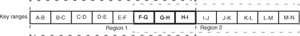
Often, if you’re willing to run through all these fixes, you can use the -repair flag rather than specify each of the previous flags individually. You can also limit the repair to particular tables by passing the table name to the repair flag (-repair MyTable).
Warning
Fixing inconsistencies in HBase tables is an advanced operational task. We encourage you to read the online manual and also try running hbck on a development environment before running it on your production cluster. Also, it never hurts to read the script’s code.
10.3.7. Viewing HFiles and HLogs
HBase provides utilities to examine the HFiles and HLogs (WAL) that are being created at write time. The HLogs are located in the .logs directory in the HBase root directory on the file system. You can examine them by using the hlog command of the bin/hbase script, like this:
$ bin/hbase hlog /hbase/.logs/regionserverhostname,60020,1340983114841/
     regionserverhostname%2C60020%2C1340983114841.1340996727020

12/07/03 15:31:59 WARN conf.Configuration: fs.default.name
is deprecated. Instead, use fs.defaultFS
12/07/03 15:32:00 INFO util.NativeCodeLoader: Loaded the
 native-hadoop librarySequence 650517 from region
     a89b462b3b0943daa3017866315b729e in table users
  Action:
     row: user8257982797137456856
     column: s:field0
     at time: Fri Jun 29 12:05:27 PDT 2012
  Action:
     row: user8258088969826208944
     column: s:field0
     at time: Fri Jun 29 12:05:27 PDT 2012
  Action:
     row: user8258268146936739228
     column: s:field0
     at time: Fri Jun 29 12:05:27 PDT 2012
  Action:
    row: user825878197280400817
    column: s:field0
    at time: Fri Jun 29 12:05:27 PDT 2012
...
...
...
The output is a list of edits that have been recorded in that particular HLog file.
The script has a similar utility for examining the HFiles. To print the help for the command, run the command without any arguments:
$ bin/hbase hfile
usage: HFile [-a] [-b] [-e] [-f <arg>] [-k] [-m] [-p] [-r <arg>] [-s] [-v]
 -a,--checkfamily    Enable family check
 -b,--printblocks    Print block index meta data
 -e,--printkey       Print keys
 -f,--file <arg>     File to scan. Pass full-path; e.g.,
                     hdfs://a:9000/hbase/.META./12/34
 -k,--checkrow       Enable row order check; looks for out-of-order keys
 -m,--printmeta      Print meta data of file
 -p,--printkv        Print key/value pairs
 -r,--region <arg>   Region to scan. Pass region name; e.g., '.META.,,1'
 -s,--stats          Print statistics
 -v,--verbose        Verbose output; emits file and meta data delimiters
Here is an example of examining the stats of a particular HFile:
$ bin/hbase hfile -s -f /hbase/users/0a2485f4febcf7a13913b8b040bcacc7/s/
     633132126d7e40b68ae1c12dead82898
Stats:
Key length: count: 1504206      min: 35 max: 42 mean: 41.88885963757624
Val length: count: 1504206      min: 90 max: 90 mean: 90.0
Row size (bytes): count: 1312480   min: 133
 max: 280  mean: 160.32370931366574
Row size (columns): count: 1312480 min: 1
 max: 2  mean: 1.1460791783493844
Key of biggest row: user8257556289221384421
You can see that there is a lot of information about the HFile. Other options can be used to get different bits of information. The ability to examine HLogs and HFiles can be handy if you’re trying to understand the behavior of the system when you run into issues.
10.3.8. Presplitting tables
Table splitting during heavy write loads can result in increased latencies. Splitting is typically followed by regions moving around to balance the cluster, which adds to the overhead. Presplitting tables is also desirable for bulk loads, which we cover later in the chapter. If the key distribution is well known, you can split the table into the desired number of regions at the time of table creation.
It’s advisable to start with fewer regions. A good place to start is the low tens of regions per RegionServer. That can inform your region size, which you can configure at a system level using the hbase.hregion.max.filesize configuration property. If you set that number to the size you want your regions to be, HBase will split them when they get to that size. But setting that number much higher than the desired region size gives you the ability to manually manage the region size and split it before HBase splits it. That means more work for the system administrator but finer-grained control over the region sizes. Managing table splitting manually is an advanced operations concept and should be done only once you’ve tried it on a development cluster and are comfortable with it. If you oversplit, you’ll end up with lots of small regions. If you don’t split in time, HBase splitting will kick in when your regions reach the configured region size, and that will lead to major compactions taking much longer because the regions would likely be big.
The HBase shell can be used to presplit regions at the time of table creation. The way to do that is to have a list of split keys in a file, with one key per line. Here’s an example:
$ cat ~/splitkeylist
A
B
C
D
To create a table with the listed keys as the split boundary, run the following command in the shell:
hbase(main):019:0> create 'mytable' , 'family',
{SPLITS_FILE => '~/splitkeylist'}
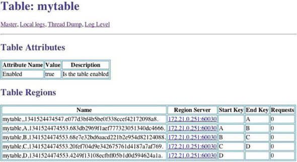
This creates a table with presplit regions. You can confirm that from your Master web UI (figure 10.10).
Figure 10.10. The HBase Master UI showing the presplit table that was created by providing the split keys at creation time. Notice the start and end keys of the regions.
Another way to create a table with presplit regions is to use the HBaseAdmin.create-Table(...) API like this:
String tableName = "mytable";
String startKey = "A";
String endKey = "D";
int numOfSplits = 5;
HBaseAdmin admin = new HBaseAdmin(conf);
HTableDescriptor desc = new HTableDescriptor(tableName);
HColumnDescriptor col = new HColumnDescriptor("family");
desc.addFamily(col);
admin.createTable(desc, startKey, endKey, numOfSplits);
We have an implementation available for you in the provided code under the utils package. It’s called TablePreSplitter.
Another implementation of creating presplit tables and even splitting them later comes packaged with HBase in the org.apache.hadoop.hbase.util.RegionSplitter class.
We’ve covered a lot of operations and management tasks in this section and equipped you with enough information to run your HBase cluster. Successful operations of a system also include the ability to handle failure scenarios of different kinds and to keep running with minimal degradation when disaster strikes. The next section explores the concept of backups in the context of HBase and where these are important.
10.4. Backup and replication
Backups tend to be one of the favorite topics of system administrators and the people responsible for operations of a system. In the world of Hadoop and HBase, the conversation changes a little. In traditional systems, backups were done to achieve redundancy in order to safeguard against system failures (hardware and/or software). Failures were considered to be something outside the system, affecting the normal operations of the system. For instance, if a relational database system goes down because the memory on the host fails, the system is unavailable until you replace the memory. If the hard disk crashes, chances are you’ll lose part or all of your data (depending on how the hard disks are configured and how many disks are being used).
Hadoop and HBase are built with failure as a first-class concern, and their design is such that they’re resilient to individual nodes failing. If a DataNode or a RegionServer host falls off the cluster, it’s no problem. Other hosts will take over the workload (stored data or regions being served), and the system will continue to function normally. The entire Hadoop stack as it exists today has high availability, which means that there is no single point of failure within the system that can bring it down or make it unavailable. Individual nodes failing isn’t a problem, but the entire data center hosting your cluster going down will cause the system to go down because Hadoop and HBase don’t span multiple data centers as of today.[11] But if your requirement is to safeguard against that kind of failure, you need some sort of a backup strategy in place.
11 The high network latency between data centers make it impractical. The alternative is to run a replica cluster in another data center. Replicas are covered in the following subsection.
Another reason to have a separate copy of the data available is to do offline processing. As we recommended in chapter 9, collocating real-time and batch-processing workloads on the same HBase cluster impacts the latencies and the performance of the cluster for both the access patterns (as compared to running them independently). By having a second copy of data in another cluster, you can segregate the online access pattern from the batch-processing access pattern and have both of them perform optimally.
There are various ways of achieving backups or second copies of the data, and each has different properties.
10.4.1. Inter-cluster replication
Replication as a feature has been in an experimental state until recently, and only savvy users have used it in production. Active development and more user demand are getting the feature to a more stable state. You don’t necessarily have to understand the ins and outs of how replication works, but we recommend that you have a good understanding of it if you plan to use it in production.
One way to copy data from one cluster to another is by replicating the writes as they come into the first cluster. This is a common operating mechanism for relational database systems. Inter-cluster replication in HBase is achieved by log shipping and is done asynchronously. That means the replication is done by sending the edits (Puts and Deletes) that go into the HLog at the time of writes to the secondary cluster to which they have to be replicated. The write to the first cluster doesn’t block on the edits being replicated. The replication happens asynchronously after the writes are done and therefore can be done across data centers because it doesn’t affect the latencies of the writes when they take place.
The instructions and descriptions of replication in this section are true for the Apache HBase 0.92.1 or the CDH4u0 releases. Given that this is a relatively new feature that hasn’t seen a lot of production usage until now, there will still be active development and the addition of new features in the near term. We encourage you to look at the release notes of the release you’re using and not take our description as set in stone.
You configure replication at a column-family level by setting the replication scope to 1 at table-instantiation time or by altering the table:
hbase(main):002:0> create 'mytable', {NAME => 'colfam1',
REPLICATION_SCOPE => '1'}
This configures the column family colfam1 to replicate to the secondary cluster when data is written to it. The same table name and column family must exist on the secondary cluster. HBase won’t create it if it doesn’t exist, and replication will fail.
Inter-cluster replication can be of three types:
- Master-slave—In this method of replication, all the writes go to only one primary cluster (master) and are replicated to the secondary
cluster (slave), as shown in figure 10.11. Nothing is ever written to the replicated column family in the secondary cluster directly. HBase doesn’t enforce this restriction
against direct writes to the replicated slave; you need to ensure this at the application level. If you by mistake end up writing to the
slave cluster, that data won’t be replicated back to the master cluster. The slave cluster can have other tables and column
families that aren’t being replicated from the master cluster.
Figure 10.11. Master-slave replication configuration, where replication happens only in a single direction
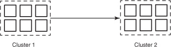
- Master-master—In master-master replication, writes received by either cluster are replicated to the other, as shown in figure 10.12.
Figure 10.12. Master-master replication scheme, where replication happens both ways. Writes to either cluster are replicated to the other cluster.
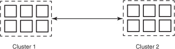
- Cyclic—In cyclic replication, you can configure more than two clusters to replicate among themselves (see figure 10.13). The replication between any two clusters can be either in master-master mode or master-slave mode. The master-master replication scheme can be considered to be a cyclic replication with only two clusters involved.
Figure 10.13. Cyclic replication scheme, where more than two clusters participate in the replication process and the relationship between any two clusters can be no replication, master-slave replication, or master-master replication
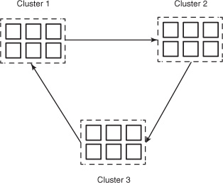
Depending on your application, you can choose which replication model will work best. If it’s only for a backup purpose or for having a second copy over which to do batch processing, the master-slave model will work fine. Master-master and cyclic replication are useful in special cases where you either want a third cluster with the same data or have data coming in from different sources into different tables and the end goal is to have an identical state across both clusters.
Configuring Inter-Cluster Replication
To configure inter-cluster replication, follow these steps:
- Put the following configuration parameter into the hbase-site.xml file of both clusters (the primary and the secondary):
<property>
<name>hbase.replication</name>
<value>true</value>
</property> After you add this configuration on all the nodes in both clusters, you need to restart the HBase daemons (RegionServer as well as Master). Keep in mind that ZooKeeper needs to be self-managed for this to work. HBase-managed Zoo-Keeper hasn’t been tested in a replication setup in HBase 0.92.1 or CDH4u0. This setting enables the cluster to participate in the replication setup. - Add secondary clusters to the list of clusters where the logs will be shipped from the primary cluster. You do so using the
add_peer command in the HBase shell. Here’s the syntax:
add_peer '<n>',
"slave.zookeeper.quorum:zookeeper.clientport:zookeeper.znode.parent" For example:
hbase(main):002:0> add_peer '1',
"secondary_cluster_zookeeper_quorum:2181:/hbase" This registers the secondary cluster as the destination where the edits need to be sent for the purpose of replication. - Set up your tables for replication. You do so at the column-family level, as explained earlier. To enable replication on existing tables, disable them, modify the column-family description, and re-enable them. Replication will start happening immediately. Ensure that the same table and column families exist on both clusters (the master and the destination slave cluster). Replication scope must be set to 1 only on the master cluster, though. Both clusters can have other tables and column families that aren’t replicated.
After setting up replication, you should verify that it’s working as desired before putting any load on the cluster.
Testing the Replication Setup
The easiest way to test that replication is working is to put a few rows into the table on the master cluster and check whether they exist on the Slave cluster. If the dataset is much larger, this may not be feasible, as can be the case if you enabled replication on a production cluster. HBase ships with a MapReduce job called VerifyReplication that you can run to compare the contents of the two tables:
$ $HBASE_HOME/bin/hbase
     org.apache.hadoop.hbase.mapreduce.replication.VerifyReplication
Usage: verifyrep [--starttime=X] [--stoptime=Y] [--families=A]
<peerid> <tablename>

Options:
 starttime    beginning of the time range
              without endtime means from starttime to forever
 stoptime     end of the time range
 families     comma-separated list of families to copy

Args:
 peerid       Id of the peer used for verification,
                 must match the one given for replication
 tablename    Name of the table to verify

Examples:
 To verify the data replicated from TestTable for a 1 hour window
     with peer #5
 $ bin/hbase org.apache.hadoop.hbase.mapreduce.replication.VerifyReplication
     --
     starttime=1265875194289 --stoptime=1265878794289 5 TestTable
But if you aren’t running the MapReduce framework, that’s not a choice. You’ll need to manage with a manual scan of the tables on the two clusters to ensure that things are working fine.
Managing Replication
There’s not much you need to do to manage replication after it’s enabled on a cluster. To stop replication in a running cluster where it’s configured, you can run the stop_replication command in the HBase shell. To start it back up, run start_replication.
A few gotchas in the current implementation make some management tasks tricky. Replication is handled at the column-family level and is configured in the active HLog file. Thus if you stop replication and then start it again, and the HLogs haven’t rolled, everything that was written between the time you stopped and restarted replication will also be replicated. This is a function of the current implementation of replication, and it may change in future releases.
To remove a peer cluster, you can use the remove_peer command with the peer ID:
hbase> remove_peer '1'
To see a list of the currently configured peers, you can use the list_peers command:
hbase> list_peers
Inter-cluster replication is an advanced feature and can make it easy to keep multiple copies of data. It’s great for maintaining two hot copies of the data: your application can switch to the secondary cluster in case something goes wrong with the primary one. The hot-failover mechanism is something you need to build into your application. This can be done purely in the application logic, or you can use DNS tricks to get the application to talk to the secondary cluster if the primary one goes down. When the primary cluster is back up and running, you can use the same DNS trick and flip back to the primary cluster.
For replication to work properly, the time on the primary and secondary clusters needs to be in sync. As we described earlier, this can be achieved using NTP. Keeping time synchronized across all nodes running HBase is important in ensuring that the system operates reliably.
The issue now is to get the newly written data from the secondary cluster back to the primary one. This can be accomplished using the CopyTable or Export/Import job, which is what we talk about next.
10.4.2. Backup using MapReduce jobs
MapReduce jobs can be configured to use HBase tables as the source and sink, as we covered in chapter 3. This ability can come in handy to do point-in-time backups of tables by scanning through them and outputting the data into flat files or other HBase tables.
This is different from inter-cluster replication, which the last section described. Inter-cluster replication is a push mechanism: new edits are pushed to the replica cluster as they come in, albeit asynchronously. Running MapReduce jobs over tables is a pull mechanism: jobs are read from the HBase tables (that is, data is pulled out) and written to a sink of your choice.
There are a couple of ways you can use MapReduce over HBase for backups. HBase ships with prebundled jobs for this purpose, as we explain in detail in appendix B. We’ll explain how you can use them for backups here.
Export/Import
The prebundled Export MapReduce job can be used to export data from HBase tables into flat files. That data can then later be imported into another HBase table on the same or a different cluster using the Import job.
The Export job takes the source table name and the output directory name as inputs. You can also give it the number of versions, start timestamp, end timestamp, and filters to have finer-grained control over what data it reads from the source table. Using the start and end timestamps can come in handy in doing incremental reads from the tables.
The data is written out efficiently in Hadoop SequenceFiles in the specified output directory, which can later be imported into another HBase table using the Import job. The SequenceFiles are keyed from rowkey to Result instances:
$ hbase org.apache.hadoop.hbase.mapreduce.Export
Usage: Export [-D<property=value>]* <tablename> <outputdir>
              [<versions> [<starttime> [<endtime>]]
                          [^[regex pattern] or [Prefix] to filter]]

  Note: -D properties will be applied to the conf used.
  For example:
   -Dmapred.output.compress=true
   -Dmapred.output.compression.codec=org.apache.hadoop.io.compress.GzipCodec
   -Dmapred.output.compression.type=BLOCK
  Additionally, the following SCAN properties can be specified
  to control/limit what is exported..
   -Dhbase.mapreduce.scan.column.family=<familyName>
Here’s an example command to export table mytable to the directory export_out:
$ hbase org.apache.hadoop.hbase.mapreduce.Export mytable export_out
12/07/10 04:21:29 INFO mapred.JobClient: Default number of map tasks: null
12/07/10 04:21:29 INFO mapred.JobClient: Setting default number of map tasks
     based on cluster size to : 12
...
...
Let’s examine the contents of the export_out directory. It should contain a bunch of output files from the map tasks:
$ hadoop fs -ls export_out
Found 132 items
-rw-r--r--   2 hadoop supergroup          0 2012-07-10 04:39 /user/hadoop/
     export_out/_SUCCESS
-rw-r--r--   2 hadoop supergroup  441328058 2012-07-10 04:21 /user/hadoop/
     export_out/part-m-00000
-rw-r--r--   2 hadoop supergroup  470805179 2012-07-10 04:22 /user/hadoop/
     export_out/part-m-00001
...
...
-rw-r--r--   2 hadoop supergroup  536946759 2012-07-10 04:27 /user/hadoop/
     export_out/part-m-00130
The Import job is the inverse of the Export job. It reads over the records in the source files, creating Put instances from the persisted Result instances. It then writes those Puts to the target table through the HTable API. Import doesn’t provide any fancy filtering or manipulation of the data along the way. If you want to perform additional manipulation, you’ll need to subclass its Importer implementation and override the map function. A simple tool has a simple invocation:
$ hbase org.apache.hadoop.hbase.mapreduce.Import
Usage: Import <tablename> <inputdir>
The command to import the table exported in the earlier example into another table named myimporttable is as follows:
$ hbase org.apache.hadoop.hbase.mapreduce.Import myimporttable export_out
Upon job completion, your target table contains the exported data.
Advanced Import with ImportTsv
Although Import is a simple complement to Export, ImportTsv is more feature-rich. It allows you to load data from newline-terminated, delimited text files. Most commonly, this is a tab-separated format, but the delimiter is configurable (for loading comma-separated files). You specify a destination table and provide it with a mapping from columns in your data file(s) to columns in HBase:
$ hbase org.apache.hadoop.hbase.mapreduce.ImportTsv
Usage: importtsv -Dimporttsv.columns=a,b,c <tablename> <inputdir>

Imports the given input directory of TSV data into the specified table.

The column names of the TSV data must be specified using the
-Dimporttsv.columns option. This option takes the form of
comma-separated column names, where each column name is either a
simple column family, or a columnfamily:qualifier. The special column
name HBASE_ROW_KEY is used to designate that this column should be
used as the row key for each imported record. You must specify exactly
one column to be the row key, and you must specify a column name for
every column that exists in the input data.

By default importtsv will load data directly into HBase. To instead
generate HFiles of data to prepare for a bulk data load, pass the
option:
  -Dimporttsv.bulk.output=/path/for/output
  Note: if you do not use this option, then the target table must
already exist in HBase

Other options that may be specified with -D include:
  -Dimporttsv.skip.bad.lines=false - fail if encountering an invalid
   line '-Dimporttsv.separator=|' - eg separate on pipes instead of
   tabs
  -Dimporttsv.timestamp=currentTimeAsLong - use the specified
   timestamp for the import
  -Dimporttsv.mapper.class=my.Mapper - A user-defined Mapper to use
 instead of org.apache.hadoop.hbase.mapreduce.TsvImporterMapper
It’s intended to be a flexible utility, allowing you even to override the Mapper class, which is used when parsing input files. You can also have ImportTsv create HFiles instead of executing Puts against the target deployment. This is called bulk import. It bypasses the HTable API, making it faster than the regular import. It does have a runtime requirement of access to the target table. ImportTsv inspects that table’s region boundaries and uses those split delimiters to decide how many HFiles to create.
Once the HFiles are created, they have to be loaded into the table. The LoadIncrementalHFiles utility, also called completebulkload, handles the messy business of installing and activating new HFiles in a table in HBase. The operation is messy because careful consideration must be given to ensure that the new HFiles match the destination table’s configuration. LoadIncrementalHFiles handles this for you by splitting any of the source HFiles so they each fit within the key-range of a single region. The HFiles are moved into place, not copied, so don’t be surprised when your source data disappears after you run this command. With your HFiles staged on the HDFS, run the tool like this:
$ hbase org.apache.hadoop.hbase.mapreduce.LoadIncrementalHFiles
usage: completebulkload /path/to/hfileoutputformat-output tablename
Let’s create a presplit table and bulk-load a tab-separated file into it:
- Create a presplit table with 10 splits:
$ for i in {1..10}; do echo $i >> splits.txt ; done
$ cat splits.txt
1
2
3
4
5
6
7
8
9
10
$ hadoop fs -put splits.txt ./
$ echo "create 'bulk_import', 'a', {SPLITS_FILE => 'splits.txt'}" | hbase shell
0 row(s) in 2.3710 seconds - Import a tab-separated file into the table. You’ll use the third column in the file as the rowkey for the HBase table. The
input tab-separated file is my_input_file, and the HFiles created will be stored in the output path hfile_output:
$ hbase org.apache.hadoop.hbase.mapreduce.ImportTsv
-
Dimporttsv.columns=a:lon,a:lat,HBASE_ROW_KEY,a:name,a:address,a:ci
ty,a:url
-Dimporttsv.bulk.output=hfile_output bulk_import ./my_input_file
12/07/10 05:48:53 INFO util.NativeCodeLoader: Loaded the native-hadoop
library
...
... - Complete the bulk load by moving the newly created HFiles into the presplit table:
$ hbase org.apache.hadoop.hbase.mapreduce.LoadIncrementalHFiles hfile_output my_bulk_import_table
CopyTable
You can use the CopyTable MapReduce job to scan through an HBase table and directly write to another table. It doesn’t create flat files of any sort. The Puts are done directly into the sink table. The sink of the CopyTable job can be another table on the same cluster or a table on an entirely different cluster. The job can also be given start and end timestamps like the Export job, which allows finer-grained control over the data being read. It also supports scenarios where source and destination HBase deployments differ—that is, with different RegionServer implementations.
Executing CopyTable involves running a MapReduce job on the source deployment and populating the destination deployment. Invocation looks like this:
$ hbase org.apache.hadoop.hbase.mapreduce.CopyTable
Usage: CopyTable [--rs.class=CLASS] [--rs.impl=IMPL] [--starttime=X]
                 [--endtime=Y] [--new.name=NEW] [--peer.adr=ADR]
                 <tablename>

Options:
 rs.class     hbase.regionserver.class of the peer cluster
              specify if different from current cluster
 rs.impl      hbase.regionserver.impl of the peer cluster
 starttime    beginning of the time range
              without endtime means from starttime to forever
 endtime      end of the time range
 new.name     new table's name
 peer.adr     Address of the peer cluster given in the format
              zookeeer.quorum:zookeeper.client.port:zookeeper.znode.parent
 families     comma-separated list of families to copy
              To copy from cf1 to cf2, give sourceCfName:destCfName.
              To keep the same name, just give "cfName"

Args:
 tablename    Name of the table to copy
Here is an example command for copying table mytable from a cluster to a remote cluster where a table with the same name exists:
$ hbase org.apache.hadoop.hbase.mapreduce.CopyTable
--peer.adr=destination-zk:2181:/hbase --families=a mytable
10.4.3. Backing up the root directory
HBase stores its data in the directory specified by the hbase.rootdir configuration property. This directory contains all the region information, all the HFiles for the tables, as well as the WALs for all RegionServers. In essence, this is where everything is persisted. But copying over this directory (using distcp) doesn’t make for a great backup solution, especially in a running system.
When an HBase cluster is up and running, several things are going on: MemStore flushes, region splits, compactions, and so on. All of these cause changes in the underlying stored data, which makes copying the HBase root directory a futile effort. Another factor that plays in is the fact that in a running system, there is data in the MemStore that hasn’t been flushed. Even if nothing else is going on, a copy of the HBase root directory doesn’t necessarily completely represent the current state of the system.
But if you stop the HBase daemons cleanly, the MemStore is flushed and the root directory isn’t altered by any process. At this moment, copying over the entire root directory could be a good point-in-time backup solution. But incremental backups still present challenges, which make this solution less viable. Restoring from the backed-up root directory is as simple as starting HBase when it’s pointing to this new root directory.
10.5. Summary
Production-quality operations of any software system are learned over time. This chapter covered several aspects of operating HBase in production with the intention of getting you started on the path to understanding the concepts. New tools and scripts probably will be developed by HBase users and will benefit you. These basic concepts of HBase operations will enable you to understand when, where, and how to use them to your advantage.
The first aspect of operations is instrumenting and monitoring the system, and that’s where we began this chapter. We covered the various monitoring systems and mechanisms and then went into the different metrics that are of interest. There are general metrics that you should monitor regardless of the workload being put on the system, and then there are metrics that are specific to the workload (read or write).
From monitoring, the chapter transitioned into talking about performance testing, measuring performance, and tuning HBase for different kinds of workloads. Performance testing is key to understanding how the cluster is tuned and what you can do to extract better performance from the cluster. Tuning HBase involves working with multiple different configuration parameters, and configurations depend on the kind of workload for which you’re planning to use your cluster.
From there we covered a list of common management tasks and how and when to do them. Some of them are common tasks that you perform more often than others, which are more specific to certain situations. The chapter concluded with backup and replication strategies, talking about the common approaches to disaster recovery and what your options are currently.
Mastering HBase operations requires an understanding of the internals and experience gained by working with the system. As much as we’d wish for HBase to be a self-tuning and self-managing system, it isn’t there yet. We hope it gets there soon, and your experience could certainly feed into that goal.