
Chapter 13: Bootstrap Forests and Boosted Trees
Perform a Bootstrap Forest for Regression Trees
Perform a Boosted Tree for Regression Trees
Use Validation and Training Samples
Introduction
Decision Trees, discussed in Chapter 10, are easy to comprehend, easy to explain, can handle qualitative variables without the need for dummy variables, and (as long as the tree isn’t too large) are easily interpreted. Despite all these advantages, trees suffer from one grievous problem: They are unstable.
In this context, unstable means that a small change in the input can cause a large change in the output. For example, if one variable is changed even a little, and if the variable is important, then it can cause a split high up in the tree to change and, in so doing, cause changes all the way down the tree. Trees can be very sensitive not just to changes in variables, but also to the inclusion or exclusion of variables.
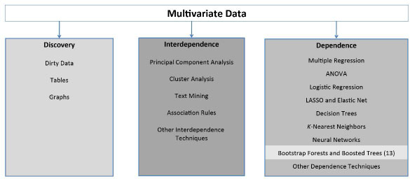
Fortunately, there is a remedy for this unfortunate state of affairs. As shown in Figure 13.1, this chapter discusses two techniques, Bootstrap Forests and Boosted Trees, which overcome this instability and many times result in better models.
Figure 13.1: A Framework for Multivariate Analysis
Bootstrap Forests
The first step in constructing a remedy involves a statistical method known as “the bootstrap.” The idea behind the bootstrap is to take a single sample and turn it into several “bootstrap samples,” each of which has the same number of observations as the original sample. In particular, a bootstrap sample is produced by random sampling with replacement from the original sample. These several bootstrap samples are then used to build trees. The results for each observation for each tree are averaged to obtain a prediction or classification for each observation. This averaging process implies that the result will not be unstable. Thus, the bootstrap remedies the great deficiency of trees.
This chapter does not dwell on the intricacies of the bootstrap method. (If interested, see “The Bootstrap,” an article written by Shalizi (2010) in American Scientist. Suffice it to say that bootstrap methods are very powerful and, in general, do no worse than traditional methods that analyze only the original sample, and very often (as in the present case) can do much better.
It seems obvious, now, that you should take your original sample, turn it into several bootstrap samples, and construct a tree for each bootstrap sample. You could then combine the results of these several trees. In the case of classification, you could grow each tree so that it classified each observation—knowing that each tree would not classify each observation the same way.
Bootstrap forests, also called random forests in the literature, are a very powerful method, probably the most powerful method, presented in this book. On any particular problem, some other method might perform better. In general, however, bootstrap forests will perform better than other methods. Beware, though, of this great power. On some data sets, bootstrap forests can fit the data perfectly or almost perfectly. However, such a model will not predict perfectly or almost perfectly on new data. This is the phenomenon of “overfitting” the data, which is discussed in detail in Chapter 14. For now, the important point is that there is no reason to try to fit the data as well as possible. Just try to fit it well enough. You might use other algorithms as benchmarks, and then see whether bootstrap forests can do better.
Understand Bagged Trees
Suppose you grew 101 bootstrap trees. Then you would have 101 classifications (“votes”) for the first observation. If 63 of the votes were “yes” and 44 were “no”, then you would classify the first observation as a “yes.” Similarly, you could obtain classifications for all the other observations. This method is called “bagged trees,” where “bag” is shorthand for “bootstrap aggregation”—bootstrap the many trees and then aggregate the individual answers from all the trees. A similar approach can obtain predictions for each observation in the case of regression trees. This method uses the same data to build the tree and to compute the classification error.
An alternative method of obtaining predictions from bootstrapped trees is the use of “in-bag” and “out-of-bag” observations. Some observations, say two-thirds, are used to build the tree (these are the “in-bag” observations) and then the remaining one-third out-of-bag observations are dropped down the tree to see how they are classified. The predictions are compared to the truth for the out-of-bag observations, and the error rate is calculated on the out-of-bag observations. The reasons for using out-of-bag observations will be discussed more fully in Chapter 14. Suffice it to say that using the same observations to build the tree and then also to compute the error rate results in an overly optimistic error rate that can be misleading.
There is a problem with bagged trees, and it is that they are all quite similar, so their structures are highly correlated. We could get better answers if the trees were not so correlated, if each of the trees was more of an independent solution to the classification problem at hand. The way to achieve this was discovered by Breiman (2001). Breiman’s insight was to not use all the independent variables for making each split. Instead, for each split, a subset of the independent variables is used.
To see the advantage of this insight, consider a node that needs to be split. Suppose variable X1 would split this node into two child nodes. Each of the two child nodes contains about the same number of observations, and each of the observations is only moderately homogeneous. Perhaps variable X2 would split this into two child nodes. One of these child nodes is small but relatively pure; the other child node is much larger and moderately homogenous. If X1 and X2 have to compete against each other in this spot, and if X1 wins, then you would never uncover the small, homogeneous node. On the other hand, if X1 is excluded and X2 is included so that X2 does not have to compete against X1, then the small, homogeneous pocket will be uncovered. A large number of trees is created in this manner, producing a forest of bootstrap trees. Then, after each tree has classified all the observations, voting is conducted to obtain a classification for each observation. A similar approach is used for regression trees.
Perform a Bootstrap Forest
To demonstrate Bootstrap Forests, use the Titanic data set, TitanicPassengers.jmp, the variables of which are described below in Table 13.1. It has 1,309 observations.
Table 13.1: Variables in the TitanicPassengers.jmp Data Set
| Variable | Description |
| Passenger Class * | 1 = first, 2 = second, 3 = third |
| Survived * | No, Yes |
| Name | Passenger name |
| Sex * | Male, female |
| Age * | Age in years |
| Siblings and Spouses * | Number of Siblings and Spouses aboard |
| Parents and Children * | Number of Parents and Children aboard |
| Ticket # | Ticket number |
| Fare * | Fare in British pounds |
| Cabin | Cabin number (known only for a few passengers) |
| Port * | Q = Queenstown, C = Cherbourg, S = Southampton |
| Lifeboat | 16 lifeboats 1–16 and four inflatables A–D |
| Body | Body identification number for deceased |
| Home/Destination | Home or destination of traveler |
You want to predict who will survive:
1. Open the Titanic Passengers.jmp data set.
2. In the course of due diligence, you will engage in exploratory data analysis before beginning any modeling. This exploratory data analysis will reveal that Body correlates perfectly with not surviving (Survived), as selecting Analyze ▶ Tabulate (or Fit Y by X), for these two variables will show. Also, Lifeboat correlates very highly with surviving (Survived), because very few of the people who got into a lifeboat failed to survive. So use only the variables marked with an asterisk in Table 13.1.
3. Select Analyze ▶ Modeling ▶ Partition.
4. Select Survived as Y, response. The other variables with asterisks in Table 13.1 are X, Factor.
5. For Method, choose Bootstrap Forest. Validation Portion is zero by default. Validation will be discussed in Chapter 14. For now, leave this at zero.
6. Click OK.
Understand the Options in the Dialog Box
Some of the options presented in the Bootstrap Forest dialog box, shown in Figure 13.2, are as follows:
● Number of trees in the forest is self-explanatory. There is no theoretical guidance on what this number should be. But empirical evidence suggests that there is no benefit to having a very large forest. 100 is the default. Try also 300 and 500. Probably, setting the number of trees to be in the thousands will not be helpful.
● Number of terms sampled per split is the number of variables to use at each split. If the original number of predictors is p, use √p rounded down for classification, and for regression use p/3 rounded down (Hastie et al. 2009, p. 592). These are only rough recommendations. After trying √p, try 2√p and √p/2, as well as other values, if necessary.
● Bootstrap sample rate is the proportion of the data set to resample with replacement. Just leave this at the default 1 so that the bootstrap samples have the same number of observations as the original data set.
◦ Minimum Splits Per Tree and Maximum Splits Per Tree are self-explanatory.
◦ Minimum Size Split is the minimum number of observations in a node that is a candidate for splitting. For classification problems, the minimum node size should be one. For regression problems, the minimum node size should be five as recommended by Hastie et al. (2009, page 592).
◦ Do not check the box Multiple Fits over number of terms. The associated Max Number of Terms is only used when the box is checked. The interested reader is referred to the user guide for further details.
Figure 13.2: The Bootstrap Forest Dialog Box

For now, do not change any of the options and just click OK.
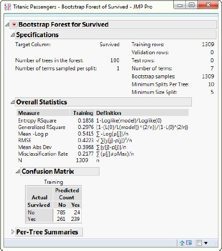
The output of the Bootstrap Forest should look like Figure 13.3.
Figure 13.3: Bootstrap Forest Output for the Titanic Passengers Data Set
Select Options and Relaunch
Your results will be slightly different because this algorithm uses a random number generator to select the bootstrap samples. The sample size is 1,309. The lower left value in the first column of the Confusion Matrix, 261, and the top right value in the right-most column, 24, are the classification errors (discussed further in Chapter 14). Added together, 261 + 24 = 285, they compose the numerator of the reported misclassification rate in Figure 13.3: 285/1309 = 21.77%. Now complete the following steps:
1. Click the red triangle next to Bootstrap Forest for Survived.
2. Select Script ▶ Relaunch Analysis.
3. The Partition dialog box appears. Click OK.
4. Now you are back in the Bootstrap Forest dialog box, as in Figure 13.2. This time, double the Number of Terms Sampled Per Split to 2.
5. Click OK.
The Bootstrap Forest output should look similar to Figure 13.4.
Figure 13.4: Bootstrap Forest Output with the Number of Terms Sampled per Split to 2

Examine the Improved Results
Notice the dramatic improvement. The error rate is now 16.5%. You could run the model again, this time increasing the Number of Terms Sampled Per Split to 3 and increasing the Number of Trees to 500. These changes will again produce another dramatic improvement. Notice also that, although there are many missing values in the data set, Bootstrap Forest uses the full 1309 observations. Many other algorithms (for example, logistic regression) have to drop observations that have missing values.
An additional advantage of Random Forests is that, just as basic Decision Trees in Chapter 10 produced Column Contributions to show the important variables, Random Forests produces a similar ranking of variables. To get this list, click the red triangle next to Bootstrap Forest for Survived and select Column Contributions. This ranking can be especially useful in providing guidance for variable selection when later building logistic regressions or neural network models.
Perform a Bootstrap Forest for Regression Trees
Now briefly consider random forests for regression trees. Use the data set MassHousing.jmp in which the target variable is median value:
1. Select Analyze ▶ Modeling ▶ Partition.
2. Select mvalue for Y, Response and all the other variables as X, Factor.
3. For method, select Bootstrap Forest.
4. Click OK.
5. In the Bootstrap Forest dialog box, leave everything at default and click OK.
The Bootstrap Forest output should look similar to Figure 13.5.
Figure 13.5: Bootstrap Forest Output for the Mass Housing Data Set

Under Overall Statistics, see the In-Bag and Out-of-Bag RMSE. Notice that the Out-of-Bag RMSE is much larger than the In-Bag RMSE. This is to be expected, because the algorithm is fitting on the In-Bag data. It then applies the estimated model to data that were not used to fit the model to obtain the Out-of-Bag RMSE. You will learn much more about this topic in Chapter 14. What’s important for your purposes is that you obtained RSquare = 0.879 and RMSE = 3.365058 for the full data set (remember that your results will be different because of the random number generator). These values compare quite favorably with the results from a linear regression: RSquare = 0.7406 and RMSE = 4.745. You can see that Bootstrap Forest regression can offer a substantial improvement over traditional linear regression.
Boosted Trees
Boosting is a general approach to combining a sequence of models, in which each successive model changes slightly in response to the errors from the preceding model.
Understand Boosting
Boosting starts with estimating a model and obtaining residuals. The observations with the biggest residuals (where the model did the worst job) are given additional weight, and then the model is re-estimated on this transformed data set. In the case of classification, the misclassified observations are given more weight. After several models have been constructed, the estimates from these models are averaged to produce a prediction or classification for each observation. As was the case with Bootstrap Forests, this averaging implies that the predictions or classifications from the Boosted Tree model will not be unstable. When boosting, there is often no need to build elaborate models; simple models often suffice. In the case of trees, there is no need to grow the tree completely out; a tree with just a few splits often will do the trick. Indeed, simply fitting “stumps” (trees with only a single split and two leaves) at each stage often produces good results.
A boosted tree builds a large tree by fitting a sequence of smaller trees. At each stage, a smaller tree is grown on the scaled residuals from the prior stage, and the magnitude of the scaling is governed by a tuning parameter called the learning rate. The essence of boosting is that, on the current tree, it gives more weight to the observations that were misclassified on the prior tree.
Perform Boosting
Use boosted trees on the data set TitanicPassengers.jmp:
1. Select Analyze ▶ Modeling ▶ Partition.
2. For Method, select Boosted Tree.
3. Use the same variables as you did with Bootstrap Forests. So select Survived as Y, response. The other variables with asterisks in Table 13.1 are X, Factor.
4. Click OK.
The Boosted Tree dialog box will appear, as shown in Figure 13.6.
Figure 13.6: The Boosted Tree Dialog Box

Understand the Options in the Dialog Box
The options are as follows:
● Number of Layers is the number of stages in the final tree. It is the number of trees to grow.
● Splits Per Tree is the number of splits for each stage (tree). If the number of splits is one, then “stumps” are being used.
● Learning Rate is a number between zero and one. A number close to one means faster learning, but at the risk of overfitting. Set this number close to one when the Number of Layers (trees) is small.
● Overfit Penalty helps protect against fitting probabilities equal to zero. It applies only to categorical targets.
● Minimum Split Size is the smallest number of observations to be in a node before it can be split.
● Multiple Fits over splits and learning rate will have JMP build a separate boosted tree for all combinations of splits and learning rate that the user chooses. Leave this box unchecked.
Select Options and Relaunch
For now, leave everything at default and click OK. The Bootstrap Tree output is shown in Figure 13.7. It shows a misclassification rate of 18.3%.
Figure 13.7: Boosted Tree Output for the Titanic Passengers Data Set

Using the guidance given about the options, set the Learning rate high, to 0.9.
1. Click the red triangle for Boosted Tree.
2. Select Script, and choose Relaunch Analysis. The Partition dialog box appears
3. Click OK. The Boosted Tree dialog box appears.
4. Change the learning rate to Learning rate to 0.9.
5. Click OK.
Examine the Improved Results
The Bootstrap Tree output will look like Figure 13.8, which has an error rate of 14.4%.
Figure 13.8: Boosted Tree Output with a Learning Rate of 0.9

This is a substantial improvement over the default model and better than the Bootstrap Forest models. You could run the model again and this time change the Number of Layers to 250. Because this is bigger than the default, you could have chosen 200 or 400. Change the Learning Rate to 0.4. Because this is somewhere between 0.9 and 0.1, you could have chosen 0.3 or 0.6. Change the number of Splits Per Tree to 5 (again, there is nothing magic about this number). You should get an error rate of 10.2%, which is much better than the second panel.
Boosted Trees is a very powerful method that also works for regression trees as you will see immediately below.
Perform a Boosted Tree for Regression Trees
Again use the data set, MassHousing.jmp:
1. Select Modeling ▶ Partition.
2. For Method, select Boosted Tree.
3. Select mvalue for the dependent variable, and all the other variables for independent variables
4. Click OK.
5. Leave everything at default and click OK.
You should get the Boosted Tree output as in Figure 13.9.
Figure 13.9: Boosted Tree Output for the Mass Housing Data Set

Boosting is better than the Bootstrap Forest in Figure 13.5 (look at RSquare and RMSE), to say nothing of the linear regression.
Next, relaunch the analysis and change the Learning rate to 0.9. This is a substantial improvement over the default model with an RSquare of 0.979. Finally, relaunch the analysis and change the Number of Layers to 250 and the Learning Rate to 0.5. This is nearly a perfect fit with an RSquare of 0.996. This is not really surprising, because both Bootstrap Forests and Boosted Trees are so powerful and flexible that they often can fit a data set perfectly.
Use Validation and Training Samples
When using such powerful methods, you should not succumb to the temptation to the make the RSquared as high as possible, because such models rarely predict well on new data. To gain some insight into this problem, you will consider one more example in this chapter in which you will use a manually selected holdout sample.
You will divide the data into two samples, a “training” sample that consists of, for example, 75% of the data, and a “validation” sample that consists of the remaining 25%. You will then rerun your three boosted tree models on the Titanic Passengers data set on the training sample. JMP will automatically use the estimated models to make predictions on the validation sample.
Create a Dummy Variable
To effect this division into training and validation samples, you will need a dummy variable that randomly splits the data into a 75% / 25% split:
1. Open TitanicPassengers.jmp.
2. Select Cols ▶ Modeling Utilities ▶ Make Validation Column. The Make Validation Column report dialog box will appear, as in Figure 13. 10.
Three methods present themselves: Formula Random, Fix Random, and Stratified Random. The Formula Random option uses a random function to split the sample; the Fix Random option uses a random number generator to split the sample. The Stratified Random will produce a stratified sample; use this option when you want equal representation of values from a column in each of the training, validation, and testing sets.
3. For now, click Formula Random.
Figure 13.10: The Make Validation Column Report Dialog Box

You will see that a new column called Validation has been added to the data table. You specified that the training set is to be 0.75 of the total rows, but this is really just a suggestion. The validation set will contain about 0.25 of the total rows.
Perform a Boosting at Default Settings
Run a Boosted Tree at default as before:
1. Select Analyze ▶ Modeling ▶ Partition.
2. As you did before, select Survived as Y, response, and the other variables with asterisks in Table 13.1 are X, Factor.
3. Select the Validation column and then click Validation.
4. For Method select Boosted Tree.
5. Click OK.
6. Click OK again for the options window. You are initially estimating this model with the defaults.
Examine Results and Relaunch
The results are presented in the top panel of Figure 13.11. There are 985 observations in the training sample and 324 in the validation sample. Because 0.75 is just a suggestion and because the random number generator is used, your results will not agree exactly with the output in Figure 13.11. The error rate in the training sample is 17.6%, and the error rate in the validation sample is 24.4%.
Figure 13.11: Boosted Trees Results for the Titanic Passengers Data Set with a Training and Validation Set

This strongly suggests that the model estimated on the training data predicts at least as well, if not better, on brand new data. The important point is that the model does not overfit the data (which can be detected when the performance on the training data is better than the performance on new data). Now relaunch:
1. Click the red triangle for Boosted Tree.
2. Select Script and Relaunch Analysis.
3. Click OK to get the Boosted Trees dialog box for the options, and change the learning rate to 0.9.
4. Click OK.
Compare Results to Choose the Least Misleading Model
You should get results similar to Figure 13.12, where the training error rate is 15.1% and the validation error rate is 24.4%.
Figure 13.12: Boosted Trees Results with Learning Rate of 0.9

Now you see that the model does a better job of “predicting” on the sample data than on brand new data. This makes you think that perhaps you should prefer the default model, because it does not mislead you into thinking you have more accuracy than you really do.
See if this pattern persists for the third model. Observe that the Number of Layers has decreased to 19, even though you specified it to be 50. This adjustment is automatically performed by JMP. As you did before, change the Learning Rate to 0.4. You should get similar results as shown in Figure 13.13, where the training error rate is 16.7% and the validation error rate is 23.5%. JMP again has changed the Number of Layers from the default 50 to 21.
Figure 13.13: Boosted Trees Results with and Learning Rate of 0.4

It seems that no matter how you tweak the model to achieve better “in-sample” performance (that is, performance on the training sample), you always get about a 20% error rate on the brand new data. So which of the three models should you choose? The one that misleads you least? The default model, because its training sample performance is close to its validation sample performance? This idea of using “in-sample” and “out-of-sample” predictions to select the best model will be fully explored in the next chapter.
The 24-year-old male passenger described above is not predicted to survive. This is how the prediction is made. Predictions are created in the following way for both Bootstrap Forests and Boosted Trees. Suppose 38 trees are grown. The data for the new case is dropped down each tree (just as predictions were made for a single Decision Tree), and each tree makes a prediction. Then a “vote” is taken of all the trees, with a majority determining the winner. If, of the 38 trees, 20 predict “No” and the remaining 18 predict “Yes,” then that observation is predicted to not survive.
Exercises
1. Without using a Validation column, run a logistic regression on the Titanic data and compare to the results in this chapter.
2. Can you improve on the results in Figure 1?
3. How high can you get the RSquare in Mass Housing example used in Figure 4?
4. Without using a validation column, apply logistic regression, bootstrap forests, and boosted tree to the Churn data set.
5. Use a validation sample on boosted regression trees with Mass Housing. How high can you get the RSquared on the validation sample? Compare this to your answer for question (3).
6. Use a validation sample, and apply logistic regression, bootstrap forests, and boosted trees to the Churn data set. Compare this answer to your answer for question (4).