This is an historical example which has been used in many textbooks. It is rather simple and shows a simple reasoning.

Let's say we look at our garden and see the grass is wet. We want to know why the grass is wet. There are two possibilities: either it was raining before or we forgot to turn off the sprinkler. Moreover, we can observe the sky. If it's cloudy, chances are it was raining before. However, if it was cloudy then presumably we didn't turn on the sprinkler, so it is more likely, in this case, we would have not forgotten to turn off the sprinkler.

This is a little example of causal reasoning that can be represented by a PGM. We identify four random variables: cloudy, sprinkler, rain, and wetgrass. Each of them is a binary variable.

We can give prior probabilities to each of them. For example, P(cloudy=true) = P(cloudy=false)=0.5.

For the other variables, we can set up conditional probability tables. For example, the rain variable could be defined as follows:

We let the reader imagine what the other probability tables would be.

The PGM for this model is:

One way to represent medical knowledge is to link symptoms to causes. The reasoning behind it is to say that causes will generate symptoms that can be observable. The problem is that there are many symptoms and many of them can have a common cause.

The idea of a PGM representing a medical knowledge base is to have two layers of nodes: one for the causes, and one for the symptoms.

The conditional probability tables associated with each node will strengthen or weaken the link between symptoms and causes so as to better represent the most likely cause of an observed symptom.

Depending on the degree of complexity of the associations, this kind of model can be a good candidate or not for exact inference.

Moreover, representing large probability tables can be a problem because there are too many parameters to determine. However, using a database of facts, it is possible to learn the parameters. In the next chapter we will see how to learn parameters.

The PGM is represented as follows:

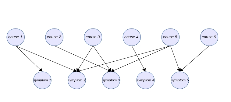
In this example, we see that symptom 2 and symptom 3 have three parents. In a more realistic medical model, it could be way more. For example, the headache symptom is caused by many different causes. In this case, it is not unusual to represent the conditional probability table associated with this node by an approximate version of it. One popular model is called the Noisy-OR model.

Unlike the previous example, it makes sense in many applications to have a deeper causal reasoning and have causes and consequences layered on top of each other. It usually helps to understand the structure of the problem.

In these kinds of model, there is no theoretical limit to the complexity of the model, but we generally advise keeping the relationships simple between nodes. For example, it's a good practice for a node not to have more than three parents. If this is the case, then it is good to study the relationships in slightly more detail to see if, by any chance, the model could be decomposed a little further.

For example in J. Binder, D. Koller, S. Russell, and K. Kanazawa, Adaptive Probabilistic Networks with Hidden Variables. Machine Learning, 29(2-3):213-244, 1997, a model is developed for estimating the expected claim costs for a car insurance policyholder.

In this model a more layered approach is adopted to represent knowledge about car insurance. The following graph shows the model. Hidden nodes are shaded and output nodes are shown with heavy lines:

Sometimes, the model can become very complex, but is nevertheless still usable. For example in S. Andreassen, F. V. Jensen, S. K. Andersen, B. Falck, U. Kjærulff, M. Woldbye, A. R. Sørensen, A. Rosenfalck, and F. Jensen, MUNIN - an Expert EMG Assistant. In Computer-Aided Electromyography and Expert Systems, Chapter 21. Elsevier (Noth-Holland), 1989., a complex network has been designed.

We show here a representation taken from the bnlearn R package (http://www.bnlearn.com/) in which the PGM is particularly big.

The reader will note that the bnlearn R package is available on the CRAN repository and can be installed just like any other package.

The following figure shows the model developed in the aforementioned paper. The model has 1,041 nodes and 1,397 edges.

Obviously setting all the parameters by hand is impossible and this kind of PGM needs to be learned from data. But it is an interesting example of a complex model:

The tree-structured PGM is an interesting model because it usually leads to a very efficient inference. The idea is simply to model the relationship between variables such as a tree, where each node will have one parent but can have many children.

So for any variable in the model, we are always representing a simple relationship that can be encoded with P(X | Y).

The following graph shows one example of such a model:

In this model, the clusters of nodes generated by the junction tree algorithm will always be made up of two nodes only: the child and its parent. So this model keeps the complexity of the junction tree algorithm low and allows for fast inference.

Of course, all these models can also be joined together to form more complex models if needed by the applications. These are just examples, and the reader is encouraged to develop his or her own models. One way to start is to understand what the causal relationships are between the variables of interest.

Also structural knowledge of the domain can be exploited to design new models. A step-by-step approach is always a good idea. One starts with a very simple model with just a few nodes and performs experiments with it to see if the model performs well. Then the model can be extended.

The problem of setting the parameters of such models is large and in the next chapter we will explore an algorithm to learn parameters from data, thus making it easier to develop an efficient PGM.