One immense benefit of going Bayesian when doing a linear model is to have better control of the parameters. Let's do an initial experiment to see what happens when the parameters are completely out of control.

We are going to generate a simple model in R and look at the parameters when they are fitted with the standard approach for linear models.

Let's first generate some data points at random to obtain 10 variables and plot them:

N <- 30
x <- runif(N, -2, 2)
X <- cbind(rep(1, N), x, x^2, x^3, x^4, x^5, x^6, x^7, x^8)
matplot(X, t='l')

Next we generate the dependent variable following the model:

y = Xβ + ϵ

Here, ϵ is a Gaussian noise of variance σ₂. We use the following code in R and plot the variable y. As we use randomly generated numbers, your plot might be different from the one in this book:

sigma <- 10
eps <- rnorm(N, mean = 0, sd = sigma)
y <- X %*% true_beta + eps
plot(y, t='l')

Then we estimate the coefficients of the model with the lm() function:

model <- lm(y~., data=data.frame(X[,2:ncol(X)]))
beta_hat <- model$coefficients

We plot the true coefficients and the estimated coefficients to see, visually, how close they are. And the result is … not good!

If we have a closer look at the values, we can clearly see that the model tried to use all the variables when we gave them a zero coefficient in the true model. Moreover, it tried to compensate between all the variables, hence the positive and negative values all along the vector of parameters. Your results might be different from the values shown here, because we use random data, but the behavior will be similar:

> true_beta
[1] 10 -3  0  8  0  0  0  0  0
> beta_hat
(Intercept)           x          V2          V3          V4          V5       V6          V7          V8
  10.012121  -30.091272    8.904295   62.005179  -12.913125  -28.102293
   
   6.844616    4.410177   -1.154756

In fact, most of the values are terribly wrong. This is a perfect example of over-fitting. The model tried to fit the data perfectly, ending in something completely off:

> true_beta
[1] 10 -3 0 8 0 0 0 0 0
> beta_hat
(Intercept) x V2 V3 V4 V5 V6 V7 V8
10.012121 -30.091272 8.904295 62.005179 -12.913125 -28.102293
6.844616 4.410177 -1.154756

In this case, we knew the true values beforehand but, in practice, we try to fit a model on a dataset to find out good values for the parameters. As we saw in the previous section, one good technique is called regularization and it is equivalent to placing prior distribution on the parameters. By doing so, we somehow constrain the parameters to stay within an acceptable range of values, with a higher probability.

Before going further, we need to visualize the structure of a linear mode and better understand the relationships between variables. We can, of course, represent it as a probabilistic graphical model.

The linear model captures the relationships between observable variables x and a target variable y. This relation is modeled by a set of parameters θ. But remember the distribution of y for each data point indexed by i:

yi ~ N(X_iβ, σ²)

Here, X_i is a row vector for which the first element is always 1 to capture the intercept of the linear model. If you look at earlier pages in this chapter, you will realize that the linear model has been written with many different forms that are all equivalent. We leave it to the reader as an exercise to show they are all equivalent. For example, X_i could be a column vector, and so on.

So our first graphical model could be as follows:

The parameter θ is itself composed of the intercept, the coefficients β for each component of X, and the variance σ² in the distribution of y_i.

So, this decomposition leads us to a second version of the graphical model in which we explicitly separate the components of θ:

We introduce again plate notation in probabilistic graphical models. When a rectangle is drawn around a set of nodes with a number or a variable in a corner (N for example), it means the same graph is repeated many times.

The likelihood function of a linear model is:

This form is representable as a graphical model and, based on the previous graph, we finally have:

In this graph, it is clearly stated that each y_i is dependent on one x_i. It is also clear that the parameters θ = {β,σ} are all shared as they are outside the plate.

For the sake of simplicity, we will keep β as a vector, but you could also decompose it into its univariate components and use the plate notation for those:

In the last two iterations of the graphical model, we see that the parameter β could have a prior probability on it instead of being fixed. In fact, the parameter σ can also be considered as a random variable. For the time being, we will keep it fixed.

Many prior distributions could be used for β but they need to be tractable or simply have an appropriate meaning in the context of a linear regression. Here we need a distribution that has a zero mean, is symmetric, and has an infinite support. The reasons are:

Given all these reasons, the Gaussian distribution seems to be a good candidate for our purpose.

The conditional distribution for y is as usual:

We remember we saw that the Maximum Likelihood Estimator (MLE) is:

And the estimator for the variance can also be estimated (left as an exercise) and is:

The good thing about having a Gaussian prior on the parameters is that it is conjugate to the likelihood function. It means that the posterior of the parameters is also a Gaussian distribution such that:

Here:

Here we find again the τ parameter, which controls how large the prior is on the parameters. It is the same parameter τ we used in the previous section on ridge regression. In fact, it can be shown that having Gaussian priors on the parameter β and the ridge regression are equivalent. The reader is encouraged to take the previous two formulas and calculate again the ridge regression to see the relation between the two.

Finally, the last thing we need to do is to compute the posterior predictive distribution. The posterior predictive distribution is the distribution of an unknown y when some Xs have been observed after computing the parameters. It is basically making a prediction with a model that has been learned with the previous method.

The reason it is important is because we do a complete Bayesian treatment of the problem, instead of a pure statistical one. In the standard linear model, the scalar product of X and β is sufficient to compute the expected value of y when we wish to make a prediction.

In other words, after finding the β parameters we simply do:

But because here we have a full Bayesian model, instead of just having the expectation of y, we have the full probability distribution. As we will see, the posterior distribution is also a Gaussian, and a Gaussian is defined by its mean and variance. Therefore, by using a full Bayesian model, we also compute the posterior variance and have an estimation of the uncertainty of the prediction:

Here:

X' and y' are respectively the new observed data upon which we want to do the prediction y'.

Finally, we can draw the graphical model for the full Bayesian interpretation of the linear model:

In fact, we only presented the case when the prior on β is Gaussian, but other priors such as a Laplace distribution can be used. This leads to an L1-penalization that doesn't have an analytical form. However, a very efficient algorithm called the Lasso can be used to find the parameters. A very efficient implementation of it can be found in the glmnet package.

Let's take an example from the beginning of this chapter again. When we tried to compute the parameters, we found strange values that were seriously off from their true value, meaning there was a problem in the estimation procedure. We saw that this problem is called over-fitting.

Then we looked at a solution by interpreting the linear model in the Bayesian framework and calculated the solutions of the problem.

Implementing it is really easy when the priors on the parameters are Gaussian:

dimension <- length(true_beta)
lambda <- diag(0.1, dimension, dimension)
posterior_sigma <- sigma^2 * solve(t(X) %*% X + sigma^2 * lambda)
posterior_beta  <- sigma^(-2) * as.vector(posterior_sigma %*% (t(X) %*% y))

The posterior parameters are now:

 posterior_beta
[1]  7.76069781 -0.06509725  1.18834799  2.72321814  0.16637478  2.65759764
[7] -0.10993147 -0.31961733  0.02273269

This is far better than what we had before. But it is still not perfect. Indeed, the true β parameters are:

true_beta <- c(10, -3, 0, 8, 0, 0, 0, 0, 0)

And we can see that the second parameter is too small and many parameters are too high, with values going from 1 to 2 when they should be zero.

Indeed, the penalization in the form of the lambda variable is too weak. It means the variance is too large. We can therefore give more penalization by doing:

lambda <- 0.5 * diag(0.1, dimension, dimension)

We then recompute the results:

 posterior_beta
[1]  9.6677088 -0.7393309  1.1248994  3.5526708 -0.1869873  2.8805658 -0.3506464
[8] -0.4582813  0.1190531

It is not perfect but the intercept is now closer to 10 (9.66) and the second parameter now has a better value. The other parameters are still off but they are going in the right direction.

We can penalize even more and run the same code again:

lambda <- 0.1*diag(0.1, dimension, dimension)
posterior_sigma <- sigma^2 * solve(t(X) %*% X + sigma^2 * lambda)
posterior_beta  <- sigma^(-2) * as.vector(posterior_sigma %*% (t(X) %*% y))
posterior_beta
[1] 12.0750175 -3.8736938  0.6105363  8.0942494 -1.0959572  1.3938047 -0.1099443
[8] -0.3496412  0.1280143

Despite it not being perfect, we see that we are closer to the true solution. Needless to say, the example we used has been specifically made to be hard to solve. Despite this, the Bayesian solution is able to converge to the true solution, where the simple linear regression was completely wrong.

After running the previous model, we can plot the results with the following code:

t <- seq(-2,2,0.01)
T <- cbind(rep(1, N), t, t^2, t^3, t^4, t^5, t^6, t^7, t^8)

plot(x,y, xlim=c(-2,2), ylim=range(y, T%*%true_beta))
lines(t,T%*%true_beta, col='black', lwd=3)
lines(t,T%*%beta_hat,  col='blue',  lwd=3)
lines(t,T%*%posterior_beta, col='red', lwd=3)

legend('topleft', c('True function', 'OLS estimate', 'Bayesian estimate'), col=c('black','blue','red'), lwd=3)

The first two lines generate evenly spaced data points to draw the results. Then the first plot draws the dataset (little black circles). Then we draw three curves on it:

The blue curve (OLS estimate) tries to follow the data points as much as possible, fitting more noise and being far away from the true function. This is a good example of over-fitting.

On the contrary, the red curve (Bayesian estimate) did a good job finding the true function that generated the data in the beginning:

Now we want to add to this graph the 95% posterior predictive interval. Thanks to the Bayesian approach, we can easily compute it from the posterior distribution. Therefore the code in R will be as follows:

pred_sigma <- sqrt(sigma^2 + apply((T%*%posterior_sigma)*T, MARGIN=1, FUN=sum))
upper_bound <- T%*%posterior_beta + qnorm(0.95)*pred_sigma
lower_bound <- T%*%posterior_beta - qnorm(0.95)*pred_sigma

The previous code computes the upper and lower bound along the dataset we used. And finally the following code draws the plot:

plot(c(0,0),xlim=c(-2,2), ylim=range(y,lower_bound,upper_bound),col='white')
polygon( c(t,rev(t)), c(upper_bound,rev(lower_bound)), col='grey', border=NA)
points(x,y)
lines(t,T%*%true_beta, col='black', lwd=3)
lines(t,T%*%beta_hat,  col='blue',  lwd=3)
lines(t,T%*%posterior_beta, col='red', lwd=3)
legend('topleft', c('True function', 'OLS estimate', 'Bayesian estimate'), col=c('black','blue','red'), lwd=3)

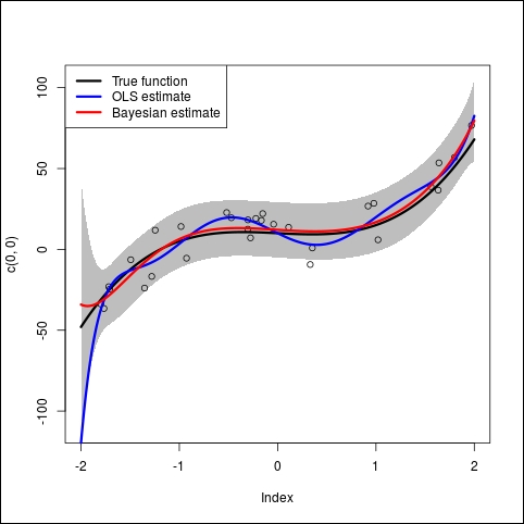
In this code we use the polygon function to draw the gray area representing the 95% predictive interval. We use the qnorm function to compute the values and you can play with theses values to change the interval.

In the previous implementation, we used the solve() function from R, but it is not always a good idea to inverse a matrix directly as it can quickly lead to numerical instability. As a quick example, here is a little piece of code that generates random invertible matrices and computes the Froebenius distance between an identity matrix and the result of the random matrix multiplied by its inverse. If M is a matrix and M^-1 its inverse, then M.M^-1=I. We see in this little example that it is not numerically the case:

N <- 200
result <- data.frame(i=numeric(N),fr=numeric(N))

for(i in 2:N)
{
        x <- matrix(runif(i*i,1,100),i,i)
        y <- t(x)%*%x

        I <- y%*%solve(y)
        I0 <- diag(i)

        fr <- sqrt(sum(diag((I-I0)%*%t(I-I0))))
        result$i[i] <- i
        result$fr[i]<- fr
}

The code generates square matrices of size going from 2 x 2 to 200 x 200 and computes the Froebenius distance between a perfect identity matrix and the identity matrix obtained by multiplying the random matrix with its inverse. Plotting the result shows that the distance is not zero all the time:

In fact, it increases with the size of the matrix, when more errors accumulate. If we plot the log of the distance, we clearly see the error getting bigger:

With a perfect inverse matrix, the distance would be zero all the time and therefore the log would be—infinite. So this simple example tells us that in Bayesian linear regression we can have problems when inverting the matrix X. We therefore need a better algorithm.

Here we present a simple algorithm to solve the ridge regression problem with a numerically stable solution. The idea is to transform the problem of matrix inversion into a simpler problem to solve, where the matrix to inverse is triangular.

If X is the matrix containing the data points, and y the vector containing the target, the idea is to first extend the matrix and the vector y as follows:

and where and

The next step is to do a QR decomposition of and the last step is to compute the inverse of R, which is easier because it's an upper triangular matrix. Finally, the coefficients of the linear regression are given by:

The algorithm in R can be implemented as follows:

# the numerically stable function
ridge <- function(X,y,lambda)
{
    tau <- sqrt(lambda)
    Xhat <- rbind(X,(1/tau)*diag(ncol(X)))
    yhat <- c(y,rep(0,ncol(X)))
 
    aqr <- qr(Xhat)
    q <- qr.Q(aqr)
    r <- qr.R(aqr)
 
    beta <- solve(r)%*% t(q) %*% yhat
 
    return(beta)
}

This algorithm returns a vector of coefficients, where the first value is the intercept. We assume here that the matrix X has a column of one on the left-hand side. We use the qr() function from R to do the QR decomposition.

The following code runs an example:

set.seed(300)
N <- 100
 
# generate some data
x <-runif(N,-2,2)
beta <- c(10,-3,2,-3,0,2,0,0,0)
X <- cbind(rep(1,length(x)), x, x^2, x^3,x^4,x^5,x^6,x^7,x^8)
y <- X %*% beta + rnorm(N,0,4)

First of all, we generate random data. The reader will note that for the first time we set the random seed manually so that the following results can be exactly reproduced. The reason for that is that we want to illustrate a nice behavior of the ridge regression.

The code generates random values on the x axis, then we give the true beta coefficients, and finally we generate the data.

We also add a random Gaussian noise to the target data y so as to test the capacity of the ridge regression with respect to the standard linear regression solved by an OLS.

The X matrix has many columns but only four of them (plus the intercept) are used to generate y so we expect the linear regression to give very small coefficients to the unused columns (or even zero coefficients).

Then we run the following code to generate results and plot them:

# plot the results
t <- seq(-2,2,0.01)
Xt <- cbind(rep(1,length(t)), t, t^2, t^3,t^4,t^5,t^6,t^7,t^8)

yt <- Xt %*% beta
yridge <- Xt %*% ridge(X,y,0.9)

plot(x,y)
lines(t,yt,t='l',lwd=2,lty=2)
lines(t,yridge,col=2,lwd=2)

olsbeta <- lm(y~X-1)
olsy <- Xt %*% olsbeta$coefficients
lines(t, olsy,col=3,lwd=2)

First of all, we generate a sequence of points on the x axis, then we compute the X matrix and then the real function called yt. This is our theoretical model without noise.

The next step is to compute the ridge regression coefficients with our new ridge function as defined previously. Finally, we compute a standard OLS solution to the same problem. And we plot the results:

The figure shows the real data set as little circles. The dashed black line is the true function, the one we called our theoretical model before. It is the function without the noise. The red line is very close to the true function. This is the ridge regression. Because of the shrinkage effect of the ridge regression, it is less sensitive to the noise and gives a better solution.

However, the green line is the standard OLS function. It has a wiggly behavior because it is more sensitive to the noise. This is an illustration of the over-fitting problem. In this example, the OLS tries too hard to be close to the data and ends up with a solution that is more unstable than the ridge regression.

In order to illustrate the last point a bit more, we run a final example in which we exaggerate the noise. Instead of having a standard deviation of 4, we use the value 16, making the data very noisy:

Obviously, this is an extreme example, but we see again that the ridge regression stays closer to the true function. The OLS solution, on the other hand, became completely unstable and is totally over-fitting.

Bayesian linear regression is a well-covered topic in R and many packages implement such models. Of course we mentioned glmnet before, which implements ridge regression and Lasso. It also implements a mixture of both, called the elastic net, in which two penalty functions are used at the same time.

Another package is bayesm, which covers linear and multivariate linear regression, multinomial logit and probit, mixtures of Gaussians, and even Dirichlet process prior density estimation.

We can also mention the arm package, which provides Bayesian versions of glm() and polr() and implements hierarchical models. It is another very powerful package.

Of course, we shouldn't stop here and ought to extend our study of Bayesian models to all sorts of algorithms and prior distributions. At some point, it becomes impossible to find an analytical solution and one should use Monte-Carlo inference, as we saw in the previous chapter.