The mixture of Bernoulli is another interesting problem. As we saw earlier, the graphical model to represent such a model is always the same. Only the probability distribution functions associated to each node change compared to the previous example. The mixture of Bernoulli finds applications in particular in analyzing black and white images, where an image is made of one Bernoulli variable for each pixel. Then the goal is to classify an image, that is, to say which value of the latent variable produced it, given some observed pixels.

For example, the following (very stylized) figure represents the letter A:

In a real application, we would use more pixels. But the idea of the application is to associate the value of pixels to each value of the latent variable, each one representing a different letter. This is a simple model for character recognition.

The distribution of a Bernoulli variable is:

Now, let's say we have D Bernoulli variables. Each Bernoulli variable is parameterized by one parameter θ_i. So the likelihood of such a model can be written as:

Here, X =(x₁, …, x_D) and θ = (θ₁, …, θ_D).

If we introduce the mixture of all the variables then the joint distribution can be written as:

Here, π = (π₁, …π_D) are the mixing parameters and the distribution p is inside as:

This is in fact the same distribution as before but for a case k only.

In order to fit this model, we need now to find the log-likelihood and, as expected, its expression will not be suitable for a direct optimization. The reason is, as usual, that we introduce latent variables for which we have no observations and we therefore need to use an EM algorithm.

The log-likelihood is taken from the main joint distribution:

This is a pretty standard way of computing the log-likelihood. And, as is usually the case for mixture models, the sum inside the log cannot be pushed out. So we end up with a quite complex expression to minimize.

Now we introduce the latent variable z into the model. It has a categorical distribution with K parameters, such that:

And the joint distribution with x is as follows:

As before with the Gaussian mixture, we will write the complete data log-likelihood. This likelihood is what we would optimize if the data set were complete—that is, without latent variables:

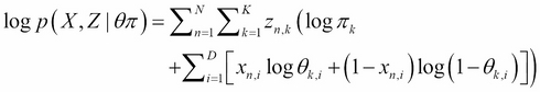
In this (very long) expression, we consider X and Z to be matrices, so in fact we use the design matrix notation, where each row vector of X (resp. Z) is one set of observations of each variable x_i (resp. z).

Using the Bayes formula, we can calculate the expectation of the complete-data log-likelihood with respect to the distribution of the latent variable. This step is necessary for the E-step of the EM algorithm, where we want to complete the data set:

And the expected value of the latent variable is:

In a sense, this is not surprising because in the end we need to compute the ratio of z_i for each subset of the dataset in which it appears after the posterior computations.

Finally, in the M-step, we can derive the complete-data log-likelihood with respect to the parameters θ_k and π and set it equal to zero. We obtain the following estimators:

Here, .

The EM algorithm will alternate between computing the expectation of z and the new values for the parameters θ and π until convergence.

This model can be extended and the same principles applied to other types of distribution—for example, a mixture of Poisson or Gamma. On the other hand, the mixture of Bernoulli can be extended to the multinomial case with the same type of derivation.

In all those models, however, we consider that we have one model for all the data point space. In other words, we somehow use the same model for the whole support of the distribution.

One extension is to consider that each subspace has its own model and therefore the choice of the sub model made by the latent variable is dependent on the data points. In Adaptive mixtures of local experts, Jacobs, R.A., Jordan, M.I, Nowlan, S.J., and Hinton, G.E. (1991) in Neural Computation, 3, 79-87, such a model is presented. We give a brief review of this interesting model in its simple form.