
6
Multiscale Modeling of Graphene-polymer Nanocomposites with Tunneling Effect
Xiaoxin LU1,2,3, Julien YVONNET2, Fabrice DETREZ2 and Jinbo BAI3
1Shenzhen Institutes of Advanced Technology, Chinese Academy of Sciences, China
2MSME, Gustave Eiffel University, Marne-la-Vallée, France
3CentraleSupélec, Paris-Saclay University , Gif-sur-Yvette, France
6.1. Introduction
The introduction of graphene-based nanomaterials has prompted the development of flexible nanocomposites for emerging applications in various fields, including energy conversion (Britnell et al. 2013), energy storage (El-Kady and Kaner 2013), electronic materials (Kim et al. 2009), sensors (Mannoor et al. 2012) and chemical screening applications (Guo et al. 2013). Graphene is among the materials with the highest in-plane electric conductivity (Novoselov et al. 2004), and its incorporation in a polymer matrix to increase the electric conductivity of almost insulating polymers is of high importance for materials-by-design. Numerous experimental and theoretical studies have reported that dispersing two-dimensional fillers such as graphene sheets in a polymer matrix can significantly improve the electric properties of the resulting composites (Liang et al. 2009, Kim and Macosko 2009, Hicks et al. 2009, Qi et al. 2011, Wang et al. 2015, He and Tjiong 2013). They exhibit an increase in several orders of magnitude of the electric conductivity, even at extremely low volume fractions of graphene sheets (Fan et al. 2012, Tkalya et al. 2014, Gao et al. 2014, Trionfi et al. 2009, Du et al. 2005), denoting the percolation phenomenon. This phenomenon can be explained by the formation of percolating paths between graphene sheets through the matrix. The percolation threshold of a random assembly of widthless discs has been evaluated in last century for the permeability problem (Charlaix 1986), dominated by the radius and number of discs. However, the introduction of nanofillers brings more complexity to the study of connectivity percolation of the composite.
Experimental works have evidenced that electrical properties of graphene or nanotube-reinforced nanocomposites are significantly dependent on the microstructure parameters, such as the size (Bryning et al. 2005) and the orientation of fillers (Yousefi et al. 2012, Du et al. 2005), as well as the inherent characteristics of the polymer matrix (Bauhofer and Kovacs 2009, Haggenmueller et al. 2007).
For design purposes, numerical models of conduction at the scale of a representative volume element (RVE) containing a significant number of graphene sheets are required to fully understand the conditions for percolation and determining optimal configurations and microstructural parameters to increase the performances of these materials. Nowadays, complete ab initio or atomistic simulations including electric conductivity in large systems like polymer–graphene reinforced composites are not feasible, and classical homogenization methods or Monte Carlo techniques (Bauhofer and Kovacs 2009, Castaneda and Willis 1995, Fan et al. 2015, Xia et al. 2017, Wang et al. 2014, Grimaldi and Balberg 2006, Otten and van der Schoot 2009) are unable to explain the nonlinear effects and low percolation thresholds in graphene–polymer nanocomposites. Simulations of larger systems require continuum descriptions of fields and related numerical methods.
In this chapter, we present a multiscale nonlinear modeling framework for graphene–polymer composites based on RVE calculations (Lu 2017, Lu et al. 2018, Lu et al. 2019). We first present a continuum framework to model the nonlinear electrical conduction at the scale of a RVE. The advantage of such model is that the microstructural parameters (volume fraction, orientation of platelets, etc.) can be changed to analyze their sensitivity with respect to the effective electrical conduction properties. The tunneling effect is taken into account to describe the nonlinear effects and low percolation thresholds observed in the literature. Then, the same model is used in structural applications. As the effective behavior of the RVE is strongly nonlinear, it is simply not possible to use an identified empirical model at the macroscopic scale. Then, a numerical two-scale approach is proposed, where the nonlinear behavior is identified by recent machine learning methods. Finally, the effect of the interphases between graphene and the polymer matrix is investigated to study its impact on the effective piezoresistive (electromechanical) behavior of the composite. A molecular dynamics (MD) approach is proposed to identify the nonlinear cohesive interfacial model.
6.2. Modeling of effective electric nonlinear behavior in graphene–polymer nanocomposites
6.2.1. Tunneling effect
Tunneling electric conductivity is a quantum phenomenon that allows electric conductivity across small isolating barriers, like thin polymer interphases between two highly conducting fillers. It has been shown that electric tunneling effect plays an important role in explaining very low percolation thresholds, as well as nonlinear electric conduction (Oskouyi et al. 2014, Sheng 1980) in such materials, especially when the characteristic distances between graphene sheets reduce to the order of nanometers. In the works of Otten and van der Schoot (2011) and Ambrosetti et al. (2010), the tunneling effect has been taken into account to analyze the percolation threshold of nanocomposites with polydisperse nanofillers, where the former focuses on carbon nanotubes and the latter extends to various particle shapes.
In a first approximation, the polymer–graphene nanocomposite can be seen as a juxtaposition of elementary graphene–polymer–graphene units (see Figure 6.1(a)). In order to understand the nonlinear electrical behavior of the nanocomposite, we first focus on the conduction mechanism of this unit. When the distance between two graphene sheets is nanoscaled, the polymer matrix can be seen as a dielectric film between two graphene electrodes. There is a strong analogy with a metal–insulator–metal device with tunnel junction. It is known that there are two types of conduction mechanisms in dielectric films (Hamann et al. 1988), which are interface-limited conduction mechanisms and bulk-limited conduction mechanism, respectively. The former depends on the electric properties at the polymer–graphene interface, while the latter depends on the electric properties of the polymer. In our work, we focus on solving the general problem and neglect the bulk-limited conduction mechanism, except Ohm’s law in varying polymers.
There are several interface-limited conduction mechanisms (Chiu 2014): (1) Schottky emission; (2) thermionic-field emission; (3) Fowler–Nordheim tunneling; (4) direct tunneling. Among them, the former two are only applied at high temperatures, when the electrons can get enough thermal energy to overcome the barrier so that the electronic current can flow in the conduction band. The latter two occur when the barrier is thin enough to permit its penetration by the quantum tunnel (Simmons 1971). To simplify the problem, we assume that the system is studied at low temperatures so that the thermal current can be neglected, and restrict the electron transportation between electrodes to the tunneling effect.
Figure 6.1 depicts the evolution of conduction band edge energy, Ec, which is at an equilibrium state across the graphene–polymer–graphene device in Figure 6.1(a).
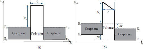
Figure 6.1. Band diagrams of graphene–polymer–polymer unit a) at equilibrium V = 0 b) with applied voltage V. The gray part indicates filling of energy levels. Ec is the conduction band edge energy and EF is the fermi level in graphene (for reasons of clarity in EF ≠ Ec, although it is the case in the graphene monolayer)
For such a 1D model of two close graphene sheets separated by a polymer matrix, the electric constitutive law is expressed in the polymer in the form
where I denotes the electric current, E is the electric field and G (E, d) is a nonlinear function of the electric field E and the distance between the two graphene sheets d. An explicit formula for the electric tunneling effect through a potential square barrier was first derived by Simmons (1963) as:
Here, the tunneling current I is a nonlinear function of electric field E and depends on three parameters: the height Φ0, width d of the barrier and the effective mass m of the electrons in graphene. This expression is obtained under the assumptions that the temperature is very low (i.e. T ≈ 0 K); the electric field E varies slowly over the width of the potential barrier (i.e. E ≈ V/d, and the rectangular barrier becomes trapezoidal under the effect of the electric field (see Figure 6.1(b))), and the trapezoidal barrier is approximated by the rectangular barrier with the same average height. This theory has been used and validated experimentally in the metal–insulator–semiconductor (Maity et al. 2016) and metal–insulator–metal capacitor field (Krishnan et al. 2008). Note that the current only comes from the electrons that cross the potential barrier. In Simmons’ model, the leakage current is not taken into account. This can be covered in the 3D extension of the conductivity model (see section 6.2.2). However, since we consider the bulk current in addition to the tunneling current, the leakage current will not affect the effective current in the composite.
6.2.2. Nonlinear electrical conduction model at the RVE scale
In this section, we describe a continuum RVE model for the graphene–polymer nanocomposite. At this scale, the graphene sheets are explicitly described at the scale of a quite large cluster of graphene nano platelets (see Figure 6.2) composed of a polymer matrix and randomly distributed and oriented graphene sheets, modeled as highly conducting imperfect interfaces (Yvonnet et al. 2008).

Figure 6.2. RVE model of the graphene-reinforced composite
The electric tunneling effect between graphene sheets described below is taken into account in the continuum model.
In this model, the total electric power of the system, ![]() , is defined by
, is defined by
where Ω ⊂ ℝ3 is the domain defining the RVE, Γ denotes the surfaces associated with graphene collectively and the density functions ωb and ωs are expressed by
where Ei(x) = −∇iø(x) = −øi(x) is the electric field, j(x) is the current density vector and ø(x) is the electric potential, where:
with ![]() as the electric conductivity tensor of the polymer matrix when neglecting the tunneling effect. In the above, the superscript s denotes surface quantities, for example, js is the surface current density. The surface electric field is defined with respect to its bulk counterpart as:
as the electric conductivity tensor of the polymer matrix when neglecting the tunneling effect. In the above, the superscript s denotes surface quantities, for example, js is the surface current density. The surface electric field is defined with respect to its bulk counterpart as: ![]() with Pij (x) = Sij − ni (x)nj (x) as a projector operator characterizing the projection of a vector along the tangent plane to Γ at a point x ∈ Γ, and n is the unit normal vector to Γ. The local constitutive relationships relating j and js with E are defined in the graphene sheets by
with Pij (x) = Sij − ni (x)nj (x) as a projector operator characterizing the projection of a vector along the tangent plane to Γ at a point x ∈ Γ, and n is the unit normal vector to Γ. The local constitutive relationships relating j and js with E are defined in the graphene sheets by
where ks denotes the surface electric conductivity of graphene and is dependent on the thickness t through:
In [6.7], kg denotes the second-order electric conductivity tensor of the bulk graphite and n is the normal vector to the graphene sheet (for more details, see Lu et al. (2018), Yvonnet et al. (2008)).
where dcut is a cut-off distance above which the tunneling effect can be neglected and G is a 3D extension of [6.2] defined by:
where Φ0 is the energy barrier height that the electrons cross and h, e and m denote Plank’s constant, the charge of an electron and a material parameter, and d is a distance function defined in 3D (see more details in Lu et al. (2018)).
Minimizing [6.3] with respect to the displacement field, and using equations [6.5]–[6.8], we obtain the weak form, which can be solved by using the finite element method (see more details in Lu et al. (2018)):
where δø ∈ H1 (Ω), δø = 0 over ∂Ω and ø ∈ H1(Ω), ø satisfying the periodic boundary conditions over ∂Ω
and where ![]() is a periodic function over Ω, such as
is a periodic function over Ω, such as ![]() .
.
The effective electric conductivity tensor ![]() is defined as:
is defined as:
where ![]() is the effective current density whose components are expressed by:
is the effective current density whose components are expressed by:
and ![]() is the effective electric field given by:
is the effective electric field given by:
6.3. Numerical simulations of effective electric conductivity
6.3.1. Effect of barrier height on the percolation threshold
Using the above model, we study the effects of barrier height between graphene and various polymers on the nonlinear response of the nanocomposite. In our simulations, we have considered that the percolation threshold corresponds to a sharp variation of the effective conductivity above 10–8 S/m. In Figure 6.3, the effective conductivity component ![]() is plotted as a function of the graphene volume fraction for the values Φ0 = 0.17 eV, 0.3 eV, 1.0 eV and without tunneling effect. The aspect ratio is η = 50 and applied electric field
is plotted as a function of the graphene volume fraction for the values Φ0 = 0.17 eV, 0.3 eV, 1.0 eV and without tunneling effect. The aspect ratio is η = 50 and applied electric field ![]() . It should be noted that for small barrier height (0.17 eV and 0.3 eV), the computation results of electric conductivity, taking into account the tunneling effect, are much larger than the predictions without tunneling effect, while for Φ0 = 1.0 eV, the effective conductivity characteristics exhibit no obvious difference, either with or without tunneling effect.
. It should be noted that for small barrier height (0.17 eV and 0.3 eV), the computation results of electric conductivity, taking into account the tunneling effect, are much larger than the predictions without tunneling effect, while for Φ0 = 1.0 eV, the effective conductivity characteristics exhibit no obvious difference, either with or without tunneling effect.

Figure 6.3. Effective conductivity versus graphene sheets volume fraction for several barrier heights Φ0,  . øc denotes the percolation threshold. Fora color version of this figure, see www.iste.co.uk/bai/nanocomposites.zip
The percolation thresholds corresponding to Φ0 =0.17, 0.3, 1.0 eV are 0.79 vol%, 0.92 vol% and 1.58 vol%, respectively. We can see from these simulations that the lower the barrier height is, the lower the percolation threshold. Experimental results reporting percolation thresholds for different polymer matrices and graphene types can be found in previous studies (Stankovich et al. 2006, Jiang et al. 2009, Ansari and Giannelis 2009, Liang et al. 2009).
6.3.2. Effect of graphene aspect ratio on the percolation threshold
Next, we use our numerical model to estimate the percolation threshold f* of the nanocomposite as a function of the graphene volume fraction and aspect ratio for graphene sheets. In Figure 6.4, the effective conductivity tensor component ![]() is computed for different aspect ratios η = 20, 50 and 100 as a function of volume fraction.
is computed for different aspect ratios η = 20, 50 and 100 as a function of volume fraction.

Figure 6.4. Effective conductivity  as a function of the graphene volume fraction for several graphene aspect ratios η,
 , Φ0 = 0.17 eV. øc denotes to the percolation threshold. For a color version of this figure, see www.iste.co.uk/bai/nanocomposites.zip
The side length of the graphene is fixed, and the various aspect ratios are obtained by changing the thickness of the graphene sheets. For each case, the values are averaged over 30 realizations of random distributions of graphene sheets within the RVE. As the behavior of the composite is nonlinear, the results of conductivity are presented for a fixed electric field ![]() . The barrier height is Φ0 = 0.17 eV. According to our numerical simulations, the effective conductivity clearly depends on the aspect ratio, a larger η provides lower percolation threshold. The obtained percolation thresholds for η = 20,50, and 100 are 1.65 vol%, 0.79 vol%, and 0.33 vol%, respectively.
. The barrier height is Φ0 = 0.17 eV. According to our numerical simulations, the effective conductivity clearly depends on the aspect ratio, a larger η provides lower percolation threshold. The obtained percolation thresholds for η = 20,50, and 100 are 1.65 vol%, 0.79 vol%, and 0.33 vol%, respectively.
6.3.3. Effect of alignment of graphene sheets
Next, we evaluate the effect of alignment of graphene sheets on the effective conductivity of the composite. For this purpose, we consider, on the one hand, a microstructure with graphene sheets whose positions and orientations are randomly distributed, and, on the other hand, a microstructure where the positions of the graphene sheets are randomly distributed, but the orientation is fixed. Each point corresponds to the mean value over 30 realizations (see realization examples in Figure 6.5).

Figure 6.5. Realizations of microscopic RVE with various graphene volume fraction. The graphene sheets are aligned parallel to the X-Y plane, and the 2D meshes on the graphene sheets are plotted. The microstructure is periodic, a graphene sheet crossing a boundary is extended on the RVE opposite side. a) 0.53 vol%, b) 0.66 vol%, c) 0.79 vol%, d) 0.92 vol%, e) 1.05 vol%, f) 1.19 vol%, g) 1.32 vol%0 and h) 1.58 vol%. For a color version of this figure, see www.iste.co.uk/bai/nanocomposites.zip
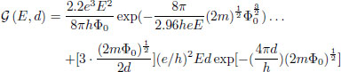
The results are presented in Figure 6.6. To clearly evidence the anisotropy, we have plotted the three components of the effective conductivity tensor. The parameters are E = 1.25 × 10⁻³ V/nm, Φ0 = 0.17 eV and η = 50.
As expected, the numerical model clearly captures the anisotropic behavior of aligned graphene sheets (see Figure 6.6(b)). Another conclusion is that aligning the graphene sheets does significantly increase either the maximum effective conductivity in the direction, normal to the graphene sheets, or the percolation threshold, as compared to randomly oriented sheets. However, the increase in conductivity after the percolation threshold is sharper in the case of aligned graphene sheets.
Finally, in Figure 6.7 we depict the current density field in the polymer matrix when tunneling effect is taken into account for aligned and randomly oriented graphene sheets to show the percolation path of electric current in both of these configurations. The parameters are η = 50 and Φ0 = 0.17 eV, f = 1.05 vol%. The electrical field is applied in the X-direction.
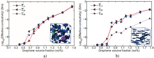
Figure 6.6. Effective conductivity tensor components as a function of the graphene volume fraction: a) random positions and orientations of graphene; b) random positions and direction of graphene normal to the Z-axis. For a color version of this figure, see www.iste.co.uk/bai/nanocomposites.zip

Figure 6.7. Current density in the polymer matrix of microstructure with graphene volume fraction f = 1.05 vol%: a) random positions and orientations of graphene; b) random positions and direction of graphene normal to the Z-axis. For a color version of this figure, see www.iste.co.uk/bai/nanocomposites.zip
6.3.4. Comparison between numerical and experimental results
In the following, the obtained numerical results are compared with available experimental data by Stankovich et al. (2006) and Zhang et al. (2010), respectively. The details of the different material and numerical parameters can be found in Lu et al. (2018). The results presented in Figures 6.8 and 6.9 show encouraging agreement between experiments and numerical simulations, even though some discrepancies exist. These disagreements can be explained as follows.

Figure 6.8. Experimentally measured (Stankovich et al. 2006) and predicted electric conductivities of polystyrene–graphene composites with various aspect ratio of graphene sheets (η = 200, 500). øc denotes the percolation threshold. For a color version of this figure, see www.iste.co.uk/bai/nanocomposites.zip

Figure 6.9. Experimentally measured (Zhang et al. 2010) and predicted electric conductivities of polyethylene terephthalate/graphene nanocomposites with various aspect ratio of graphene sheets (η = 50, 150). øc denotes the percolation threshold. For a color version of this figure, see www.iste.co.uk/bai/nanocomposites.zip
First, the dispersion state of graphene is hard to control in the experimental preparation, and the aggregation of graphene in the microstructure may lead to the heterogeneity of the macroscopic property. However, in our present work, the numerical simulation is based on randomly distributed graphene sheets. Moreover, the numerical simulation ignores the defects in the nanocomposite, especially the ones on the interface between graphene and the polymer. It should also be noted that we focus on the simulation of nanocomposites with small graphene volume fraction due to the extremely small percolation threshold that we are interested in. The simulation of electric conductivity at high graphene volume fraction calls for a large computation cost and has quite a long computation time due to the refined meshes, so we did not take this further.
6.4. Two-scale approaches
In this section, the former model is used in a structural application. Using a nonlinear model directly obtained from a full RVE simulation in a structure problem, for example, solved by finite elements, is not a trivial problem, as there is no closed form for the effective constitutive law. One direct solution is to numerically evaluate the response of the RVE at each point (Gauss points) in the structural mesh and use a Newton approach to solve the problem (FE2 method (Feyel 1999)). However, such a procedure is highly time consuming and induces intractable computational times for 3D applications. Here, we present a recent approach (Lu et al. 2019), a data-driven-based computational homogenization method based on machine learning, to describe the nonlinear electric conduction in random graphene–polymer nanocomposites. In the proposed technique, the nonlinear effective electric constitutive law is provided by a neural network surrogate model constructed through a learning phase on a set of RVE nonlinear computations. In contrast to multilevel (FE2) methods where each integration point is associated with a full nonlinear RVE calculation, the nonlinear macroscopic electric field-electric flux relationship is efficiently evaluated by the surrogate neural network model, drastically reducing (by several orders of magnitude) the computational times in multilevel calculations.
Artificial neural networks (ANNs), commonly referred to as neural networks, are massively parallel computing systems inspired by the biological neural network of the human brain, that is, an ANN model attempts to use some organizational principles used in a biological neural network, like in the human brain. Thus, ANNs are information-processing mathematical models configured to perform tasks through a learning process and have been extensively used by researchers across different disciplines in order to solve a variety of problems in pattern recognition, prediction, optimization and clustering. One of the most important features of an ANN is its ability to learn the task for which it is designed through examples, provide the network with a set of input/output signals called training samples and use it to create a mapping between the input and the output. Basically, the training of the ANN consists of ordinary steps to tune the synaptic weights so that a map that closely fits the training set is achieved. Three major learning strategies exist: (i) supervised learning, in which each training sample is composed of the input signals and their corresponding outputs, (ii) unsupervised learning, in which prior knowledge of the respective outputs is not required and (iii) reinforced learning, in which the learning algorithms adjust the weights relying on information acquired through the interaction with the model. In this work, we utilize a supervised learning strategy, which is explained in the following. In the present work, the Matlab® Neural Network Toolbox has been used.
6.4.1. Construction of the surrogate model based on ANN: strategy
The key idea of this work is to construct a surrogate model based on neural networks in a multilevel finite element framework. In the present method, called neural network computational homogenization (NN-CH), we use a multi-layer perceptron (MLP) to construct the nonlinear relationship between the (input) effective electric field vector ![]() and the (output) effective electric current density vector
and the (output) effective electric current density vector ![]() using the model described in section 6.2.2. As this relationship is not known in advance, each set of values for
using the model described in section 6.2.2. As this relationship is not known in advance, each set of values for ![]() requires a nonlinear finite element problem to be solved to obtain the corresponding
requires a nonlinear finite element problem to be solved to obtain the corresponding ![]() , as defined in section 6.2.2. To avoid these costly calculations at the macro-scale, we propose here to define this relationship through the ANN surrogate model. For this purpose, a set of data consisting of N couples of vectors
, as defined in section 6.2.2. To avoid these costly calculations at the macro-scale, we propose here to define this relationship through the ANN surrogate model. For this purpose, a set of data consisting of N couples of vectors ![]() and their corresponding
and their corresponding ![]() are provided to the neural network.
are provided to the neural network.

Figure 6.10. Off-line computational in the data-driven computational homogenization framework. For a color version of this figure, see www.iste.co.uk/bai/nanocomposites.zip
The procedure for constructing the ANN-based surrogate multiscale model is illustrated in Figures 6.10 and 6.11 and outlined in the following steps:
- 1) generate N number of electric field vectors
 to be used for the MLP training;
 - 2) run N FEM nonlinear RVE calculations, for applied effective electric field vectors
 and compute the corresponding effective current densities
  , as described in section 6.2.2;
 - 3) train the MLP using
 as inputs and
  as the corresponding outputs;
 - 4) check for accuracy of the trained MLP;
- 5) if the error (using appropriate metrics) is larger than a tolerance, add new input (through steps 1–2) to the set of data and perform steps 3–5 again.

Figure 6.11. Online computational in the data-driven computational homogenization framework
6.4.2. Structural application
One advantage of the NN-CH approach is that once the surrogate model is constructed, many structural problems can be solved without new calculations on the RVE and taking advantage of the off-line calculation costs. In this next example, we consider the structure described in Figure 6.12. The side lengths of the domain are Lx = 16 μm, Ly =8 μm, Lz = 2 μm. The diameter of the hole in the middle of the cuboid is D = 4 μm.
A mesh of 1820 tetrahedral elements is constructed. The boundary condition is ø(x = 0 μm) = 0 V, ø(x= 16 μm) = 160 V on the corresponding end surfaces. The current density ![]() on the other boundary surfaces.
on the other boundary surfaces.

Figure 6.12. Structural problem: geometry, boundary conditions and mesh. For a color version of this figure, see www.iste.co.uk/bai/nanocomposites.zip

Figure 6.13. NN-CH simulation results compared with FE2 results for the structural composite structure, with 0.53 vol% of graphene within the RVE. (a) Overall current density component Jx field and (b) Jx on slices (x = 8 μm, y = 4 μm, z = 1 μm) computed by NN-CH simulation. (c) Overall current density component Jx field, and (d) Jx on slices (x = 8 μm, y = 4 μm, z = 1 μm) computed by FE2 simulation. For a color version of this figure, see www.iste.co.uk/bai/nanocomposites.zip
Results for an RVE of 0.53 vol% are shown in Figure 6.13. For NN-CH, the calculation took 267.45 s with 12 parallel workers, against 126 h for FE2. A comparison of the different fields by FE2 is provided in Figure 6.13, showing a very good agreement. Then, we show that accurate nonlinear models based on RVE can be used in structural engineering applications at reasonable costs.
6.5. Electromechanical coupling
In this section, we introduce mechanical effects related to the graphene–polymer interface and its impact on the effective piezoresistive properties of the composite, or in other words, the effect of the mechanical response on the electrical response of the material. For this purpose, a cohesive zone model is identified by atomistic simulations. This cohesive zone model is used to enrich an imperfect interface model, which represents the graphene sheet as an effective imperfect interface. This nonlinear mechanical model is used to generate a deformed representative volume element to study the influence of strain and interfacial decohesion on the conductivity of graphene/polymer nanocomposites. The local model (RVE) employs the nonlinear electrical model described in section 6.2.2.
6.5.1. Mechanical modeling
In this section, we use the theory of nonlinear continuum mechanics at finite strains, details of which can be found in previous studies (Gurtin et al. (2010), Tadmor et al. (2012), among others). We consider the RVE described in Figure 6.2. Here, the RVE in the reference configuration Ω0 ∈ ℝ3, and the spatial configuration Ωt ∈ ℝ3.
The two sides of the interface are denoted by ![]() and
and ![]() . The unit vector normal to the interface in the reference configuration is N(X). The displacement of the bulk, and the two sides of the interface are u, u– and u+, respectively. The current positions x of the material particles at the initial position X are defined by x = X + u for the bulk. x– and x+ are the current position for the two sides of interface. The graphene sheets are modeled as general imperfect interfaces (Chatzigeorgiou et al. 2017, Javili et al. 2017), satisfying [[u]] = u+ – u– ≠ 0 and [[x]] ≠ 0; the traction through the graphene surfaces is also discontinuous, [[t]] = t+ – t– ≠ 0, where t+ and t– are, respectively, the traction on
. The unit vector normal to the interface in the reference configuration is N(X). The displacement of the bulk, and the two sides of the interface are u, u– and u+, respectively. The current positions x of the material particles at the initial position X are defined by x = X + u for the bulk. x– and x+ are the current position for the two sides of interface. The graphene sheets are modeled as general imperfect interfaces (Chatzigeorgiou et al. 2017, Javili et al. 2017), satisfying [[u]] = u+ – u– ≠ 0 and [[x]] ≠ 0; the traction through the graphene surfaces is also discontinuous, [[t]] = t+ – t– ≠ 0, where t+ and t– are, respectively, the traction on ![]() and
and ![]() associated with the normal N(X).
associated with the normal N(X).
Here, we follow the theory of imperfect interface at finite strains, developed by Javili et al. (2017). The internal virtual work, δWint, is given in reference configuration by the contributions of polymer bulk and graphene sheets, which are modeled by imperfect interfaces:
The polymer bulk contribution is
where P is the first Piola–Kirchoff stress, such as t = P · N and δF = ∇x δu is the gradient of the virtual displacement Ju with respect to the Lagrangian coordinate X. It should be noted that in this chapter, we defined (A · b)i = Aijbj , a.b = aibi, (AB)ij = Aik Bkj.
The contribution of imperfect interfaces is given by
where P(s) is surface first Piola–Kirchof stress and δF(s) = ∇X δus · ![]() denotes the surface gradient of the virtual displacement, where δus = 1/2(δu+ + δu–) is a virtual displacement field on the interface and
denotes the surface gradient of the virtual displacement, where δus = 1/2(δu+ + δu–) is a virtual displacement field on the interface and ![]() is the projector into the tangent plan of the interface in the reference configuration. {{t}} = 1/2 (t+ +1–) is the average of traction. Note that the expression of internal virtual work with imperfect interfaces is true by constraining the interface motion to the midplane (Javili et al. 2017), that is, by imposing the definition of the interface displacement us = 1/2(u+ + u–).
is the projector into the tangent plan of the interface in the reference configuration. {{t}} = 1/2 (t+ +1–) is the average of traction. Note that the expression of internal virtual work with imperfect interfaces is true by constraining the interface motion to the midplane (Javili et al. 2017), that is, by imposing the definition of the interface displacement us = 1/2(u+ + u–).
Using the second Piola–Kirchhoff stress tensor S = F–1P (respectively, the surface second Piola–Kirchhoff stress tensor, Ss = (Fs)–1 Ps with ![]() , we finally obtain the following expression of internal virtual work (for a configuration in static equilibrium):
, we finally obtain the following expression of internal virtual work (for a configuration in static equilibrium):
where δ∈ (respectively, δ∈s) is the variation of the symmetric Green–Lagrange strain tensor, ![]() (respectively, the variation of the surface Green–Lagrange strain tensor,
(respectively, the variation of the surface Green–Lagrange strain tensor, ![]() .
.
6.5.2. Constitutive laws
We choose the isotropic Saint Venant–Kirchhoff model for the bulk part, which is an extension of the linear elastic material model. The second Piola–Kirchoff stress is given by:
where the Lame’s coefficients are λ(b) = 6890 MPa and μ(b) = 680 MPa (Lu 2017). They are identified by deformation of MD simulation box of pure PE following classical procedures (Theodorou and Suter 1986).
As for the bulk, for sake of simplicity, we assume that the behavior of the imperfect interface is reversible. The surface elastic behavior of graphene is assumed to be isotropic along its tangent plane to the surface, such that the surface second Piola–Kirchoff stress is also given by the Saint Venant–Kirchhoff model:
where the surface Lame’s coefficient λ(s) = 19.0 N.m–1 and μ(s) = 18.7 N.m–1 are identified by the MD simulation (Lu 2017).
The expression of traction {{t}} is assumed to be aligned with the displacement jump [[u]] and is given by:
where gcz (·) is the function identified by the MD simulations in equation [6.27].
6.5.3. Weak form of mechanical problem
In order to relate the micro stress and strain fields to the imposed macroscopic strain, the effective quantities are defined as in Javili et al. (2017):
and
where ![]() and
and ![]() are the effective deformation gradient and effective first Piola–Kirchoff stress, respectively. The effective Green-Lagrange strain tensor
are the effective deformation gradient and effective first Piola–Kirchoff stress, respectively. The effective Green-Lagrange strain tensor ![]() and the effective second Piola–Kirchoff stress
and the effective second Piola–Kirchoff stress ![]() are defined by:
are defined by:
To impose that the incremental internal virtual work at the micro-scale, δWint, is equal to the macroscopic internal virtual work, ![]() , we chose periodic boundary conditions to satisfy the extended Hill–Mandel condition (Javili et al. 2017). The weak form associated with the mechanical problem at micro-scale is given by: find u ∈ H1(Ω0), satisfying the boundary conditions
, we chose periodic boundary conditions to satisfy the extended Hill–Mandel condition (Javili et al. 2017). The weak form associated with the mechanical problem at micro-scale is given by: find u ∈ H1(Ω0), satisfying the boundary conditions ![]() over δΩ0 with ũ periodic, such that
over δΩ0 with ũ periodic, such that

for all ![]() .
.
We use FEM to discretize the solution space, linear tetrahedrons for the bulk part and linear triangles for interfaces. A Newton–Raphson procedure is used to solve this nonlinear problem step by step for small increments ![]() of effective strain gradient.
of effective strain gradient.
6.5.4. Identification of cohesive zone model
To study the separation in opening mode, graphene is moved in successive steps of 0.5Å along the Z direction by following a minimization procedure. The graphene atoms and bottom layer of the polymer are kept fixed (see Figure 6.14(a)). The separation process is depicted in Figure 6.14. The polymer chains undergo stretch at the beginning along the Z direction, then form highly oriented structures, called fibrils or nano-fibrils. Voids appear between the fibrils during the decohesion. This deformation mechanism observed during the simulation is similar to the nano-crazes of some semi-crystalline polymers, such as polybutene (Thomas et al. 2009, Detrez 2008). The size of the void grows along the separation direction and the extended chains slide along the graphene sheet to increase the fibrils, as described in the reference review paper by Kramer and Berger (1990). It should be noted that the separation is controlled by the chain desorption at the graphene surface by sliding, which is dominated by Van der Waals interactions.
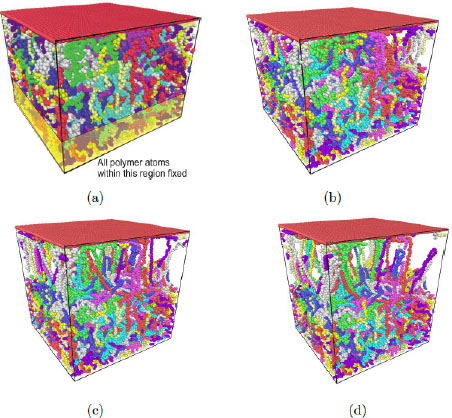
Figure 6.14. Evolution of the atomistic model during the normal separation. The model contains 44,860 atoms, and the graphene is moved with a step of 0.5 Å. The graphene atoms and the bottom layer of the polymer are fixed during the relaxation. For a color version of this figure, see www.iste.co.uk/bai/nanocomposites.zip
The average force of polymer on graphene was monitored, from which we can get the normal traction force tn of the cohesive zone as a function of the displacement of the graphene layer, [[un]], as shown in Figure 6.15. First, the force varies linearly with the displacement of the graphene sheet. Then, the curve bends to reach a maximum at 0.7 nm, called the yield threshold. This phase corresponds to the nano-fribils creation and to the cavity initiation. Once the yield threshold is crossed, the force decreases with the displacement of the graphene sheet. During this phase, the chains slip on the graphene sheet to feed the fibrils. It is interesting to note that the observed softening is related to the reduction of the contact area between the polymer chains and graphene. We propose fitting the MD results with the following empirical model:


Figure 6.15. Traction force, tn versus displacement of graphene layer [[un]]. The points denote the MD results and the line is the fitting curve. There is a correspondence between the bold points with the numbers (1–4) on the curve and the figures above. For a color version of this figure, see www.iste.co.uk/bai/nanocomposites.zip
The above model is incorporated in the mechanical model described in section 6.5.1 and is coupled with the nonlinear electrical model described in section 6.2.2.
6.5.5. Evolution of electrical properties under stretching of the composite
Using the above electro-mechanical model of nanocomposites, we study the impact of both stretching and decohesion at the graphene polymer interface on the electric conductivity. Indeed, the conductivity is controlled by the tunneling effect, which depends strongly on the distance between graphene. Therefore, we impose an macroscopic elongation, ![]() , on the RVEs, from
, on the RVEs, from ![]() . Due to the large computational times, only one RVE microstructure is randomly studied for each graphene volume fraction.
. Due to the large computational times, only one RVE microstructure is randomly studied for each graphene volume fraction.

Figure 6.16. Effective electrical conductivity of graphene reinforced nanocomposites as a function of the deformation for various graphene volume fraction. The barrier height between graphene and polymer matrix is set to 0.17 eV, and the graphene aspect ratio is 75. The applied electric field is 0.0025 V/nm. a)  , b)
, b)  and c)
  . For a color version of this figure, see www.iste.co.uk/bai/nanocomposites.zip
The deformed microstructures are stored for each 1% increment of deformation and the distance function, d(x), is updated. Introducing the new distance function, the electrical conductivities at different effective strain ![]() are shown in Figure 6.16. The boundary between the insulator and conductor is defined as 10–8 S/m (Singh 2011), below which the material is supposed to be the insulator. In the other situation, it behaves like a conductor. Focusing on the electrical conductivity along the direction of deformation
are shown in Figure 6.16. The boundary between the insulator and conductor is defined as 10–8 S/m (Singh 2011), below which the material is supposed to be the insulator. In the other situation, it behaves like a conductor. Focusing on the electrical conductivity along the direction of deformation ![]() , in Figure 6.16(a) we can observe that the mechanical deformation has little effect on the electrical conductivity of the nanocomposites when the graphene volume fraction is below the percolation threshold, f < fc = 0.52 vol%. When the graphene volume fraction is above the percolation threshold (f > fc = 0.52 vol%), the electrical conductivity
, in Figure 6.16(a) we can observe that the mechanical deformation has little effect on the electrical conductivity of the nanocomposites when the graphene volume fraction is below the percolation threshold, f < fc = 0.52 vol%. When the graphene volume fraction is above the percolation threshold (f > fc = 0.52 vol%), the electrical conductivity ![]() decreases with the applied elongation, but it should be noted that the nanocomposites remain as the conductor. However, if the graphene volume fraction is around the percolation threshold (f ≈ fc = 0.52 vol%), a sharp decrease in the electrical conductivity can be seen when the nanocomposites are subjected to strain, which is regarded as a transition point from conductor to insulator. For instance, with 0.66 vol% graphene the transition point of the sample is
decreases with the applied elongation, but it should be noted that the nanocomposites remain as the conductor. However, if the graphene volume fraction is around the percolation threshold (f ≈ fc = 0.52 vol%), a sharp decrease in the electrical conductivity can be seen when the nanocomposites are subjected to strain, which is regarded as a transition point from conductor to insulator. For instance, with 0.66 vol% graphene the transition point of the sample is ![]() , and with f = fc = 0.52 vol% graphene it is
, and with f = fc = 0.52 vol% graphene it is ![]() . We note that this drop in conductivity does not occur for any curve above a volume fraction f ≥ 0.79 vol%. However, the elongation would not affect the electrical conductivities of the nanocomposites in the transverse directions
. We note that this drop in conductivity does not occur for any curve above a volume fraction f ≥ 0.79 vol%. However, the elongation would not affect the electrical conductivities of the nanocomposites in the transverse directions ![]() and
and ![]() , which can be seen from Figures 6.16(b) and (c). This is probably a consequence of the fact that the simulations for each volume fraction have only been performed on one realization, and that some configurations might be more favorable to this effect. The results demonstrate that the graphene nanocomposite with certain graphene volume fraction (around percolation threshold) may lead to the existence of conductor to insulator behavior under finite strain. But it is also dependent on the microstructure of nanocomposite, and it only happens to those whose current path formed by graphene can be destroyed during the tension.
, which can be seen from Figures 6.16(b) and (c). This is probably a consequence of the fact that the simulations for each volume fraction have only been performed on one realization, and that some configurations might be more favorable to this effect. The results demonstrate that the graphene nanocomposite with certain graphene volume fraction (around percolation threshold) may lead to the existence of conductor to insulator behavior under finite strain. But it is also dependent on the microstructure of nanocomposite, and it only happens to those whose current path formed by graphene can be destroyed during the tension.
After observing this typical conductor-to-insulator transition for the composite with f = 0.66 vol% graphene by the proposed model, we compare the effective conductivity with the results that are estimated without considering the decohesion between graphene and the polymer matrix (i.e. we prescribe [[u]] = 0). It can be seen in Figure 6.17 that by neglecting the cohesive interface, the transition point increases from ![]() , which shows the important role of decohesion at the interface in predicting the piezoresistivity properties of polymer graphene nanocomposites. It is interesting to note that it is theoretically possible to design a composite that can go from conductor to insulator by varying the applied strain on the system. This transition can be induced mainly by the decohesion for weak interfaces, or only by strain for a stronger interface, but for a more important applied elongation.
, which shows the important role of decohesion at the interface in predicting the piezoresistivity properties of polymer graphene nanocomposites. It is interesting to note that it is theoretically possible to design a composite that can go from conductor to insulator by varying the applied strain on the system. This transition can be induced mainly by the decohesion for weak interfaces, or only by strain for a stronger interface, but for a more important applied elongation.
6.6. Conclusion
In this chapter, we have presented several recent advances in the modeling of graphene–polymer nanocomposites. First, a model at the scale of an RVE was presented, where the effects of microstructures and nonlinearities associated with the quantum tunneling effects have been taken into account. This model can be used to capture the effective nonlinear electrical properties of the composites with respect to the microstructural parameters (graphene platelets orientation, volume fraction, etc.). Then, a two-scale numerical strategy was introduced to use this model at the scale of a real structure through a numerical homogenization process involving machine learning. Finally, we have presented the effects of weak electromechanical coupling in these composites by introducing the mechanical damage behavior at the interfaces, which have been identified by molecular dynamics. These different numerical tools provide promising modeling approaches to predict and design the electro-mechanical behavior of future nanocomposites.
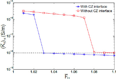
Figure 6.17. Effective electric conductivity as a function of effective strain  for the composite with 0.66 vol% graphene, both with and without considering the cohesive interface, Φo = 0.17. For a color version of this figure, see www.iste.co.uk/bai/nanocomposites.zip
6.7. References
Ambrosetti, G., Grimaldi, C., Balberg, I., Maeder, T., Danani, A., Ryser, P. (2010). Solution of the tunneling-percolation problem in the nanocomposite regime. Physical Review B, 81(15), 155434.
Ansari, S. and Giannelis, E.P. (2009). Functionalized graphene sheet-poly (vinylidene fluoride) conductive nanocomposites. Journal of Polymer Science Part B: Polymer Physics, 47(9), 888–897.
Bauhofer, W. and Kovacs, J.Z. (2009). A review and analysis of electrical percolation in carbon nanotube polymer composites. Composites Science and Technology, 69(10), 1486–1498.
Britnell, L., Ribeiro, R.M., Eckmann, A., Jalil, R., Belle, B.D., Mishchenko, A., Kim, Y., Gorbachev, R.V., Georgiou, T., Morozov, S.V., Grigorenko, A.N., Geim, A.K., Casiraghi, C., CastroNeto, A.H., Novoselov, K.S. (2013). Strong light-matter interactions in heterostructures of atomically thin films. Science, 340(6138), 1311–1314.
Bryning, M.B., Islam, M.F., Kikkawa, J.M., Yodh, A.G. (2005). Very low conductivity threshold in bulk isotropic single-walled carbon nanotube–epoxy composites. Adv. Mater., 17(9), 1186–1191.
Castaneda, P. and Willis, J. (1995). The effect of spatial distribution on the effective behavior of composite materials and cracked media. Journal of the Mechanics and Physics of Solids, 43(12), 1919–1951.
Charlaix, E. (1986). Percolation threshold of a random array of discs: A numerical simulation. Journal of Physics A: Mathematical and General, 19(9), L533.
Chatzigeorgiou, G., Meraghni, F., Javili, A. (2017). Generalized interfacial energy and size effects in composites. J. Mech. Phys. Solids, 106, 257–282.
Chiu, F.C. (2014). A review on conduction mechanisms in dielectric films. Advances in Materials Science & Engineering, 578168, 1–18.
Detrez, F. (2008). Nanomécanismes de déformation des polyméres semi-cristallins : étude in situ par microscopié à force atomique et modélisation. PhD Thesis, Université Lille I.
Du, F., Fisher, J., Winey, K. (2005). Effect of nanotube alignment on percolation conductivity in carbon nanotube/polymer composites. Physical Review B, 72(12), 121404.
El-Kady, M.F. and Kaner, R.B. (2013). Scalable fabrication of high-power graphene micro-supercapacitors for flexible and on-chip energy storage. Nature Communications, 4, 1475.
Fan, P., Wang, L., Yang, J., Chen, F., Zhong, M. (2012). Graphene/poly(vinylidene fluoride) composites with high dielectric constant and low percolation threshold. Nanotechnology, 23(36), 365702.
Fan, Z., Gong, F., Nguyen, S.T., Duong, H.M. (2015). Advanced multifunctional graphene aerogel–poly (methyl methacrylate) composites: Experiments and modeling. Carbon, 81, 396–404.
Feyel, F. (1999). Multiscale FE2 elastoviscoplastic analysis of composite structure. Computational Material Science, 16(1–4), 433–454.
Gao, C., Zhang, S., Wang, F., Wen, B., Han, C., Ding, Y., Yang, M. (2014). Graphene networks with low percolation threshold in ABS nanocomposites: Selective localization and electrical and rheological properties. ACS Applied Materials & Interfaces, 6(15), 12252–12260.
Grimaldi, C. and Balberg, I. (2006). Tunneling and nonuniversality in continuum percolation systems. Phys. Rev. Lett., 96(6), 066602.
Guo, W., Cheng, C., Wu, Y., Jiang, Y., Gao, J., Li, D., Jiang, L. (2013). Bio-inspired two-dimensional nanofluidic generators based on a layered graphene hydrogel membrane. Advanced Materials, 25(42), 6064–6068.
Gurtin, M.E., Fried, E., Anand, L. (2010). The Mechanics and Thermodynamics of Continua. Cambridge, New York.
Haggenmueller, R., Guthy, C., Lukes, J.R., Fischer, J.E., Winey, K.I. (2007). Single wall carbon nanotube/polyethylene nanocomposites: Thermal and electrical conductivity. Macromolecules, 40(7), 2417–2421.
Hamann, C., Burghardt, H., Frauenheim, T. (1988). Electrical Conduction Mechanisms in Solids. VEB Deutscher Verlag der Wissenschaften, Berlin.
He, L. and Tjiong, S.C. (2013). Low percolation threshold of graphene/polymer composites prepared by solvothermal reduction of graphene oxide in the polymer solution. Nanoscale Research Letters, 8(1), 132.
Hicks, J., Behnamand, A., Ural, A. (2009). A computational study of tunnelingpercolation electrical transport in graphene-based nanocomposites. Applied Physics Letters, 95(21), 213103.
Javili, A., Steinmann, P., Mosler, J. (2017). Micro-to-macro transition accounting for general imperfect interfaces. Comput. Methods Appl. Mech. Engrg., 317, 274–317.
Jiang, J.Y., Kim, M.S., Jeong, H.M., Shon, C.M. (2009). Graphite oxide/poly (methyl methacrylate) nanocomposites prepared by a novel method utilizing macroazoinitiator. Composites Science and Technology, 69(2), 186–191.
Kim, H. and Macosko, C.W. (2009). Processing-property relationships of polycarbonate/graphene composites. Polymer, 50(15), 3797–3809.
Kim, K.S., Zhao, Y., Jang, H., Lee, S.Y., Kim, J.M., Kim, K.S., Ahn, J.H., Kim, P., Choi, J.Y., Hong, B.H. (2009). Large-scale pattern growth of graphene films for stretchable transparent electrodes. Nature, 457(7230), 706.
Kramer, E.J. and Berger, L.L. (1990). Fundamental processes of craze growth and fracture. Polym. Sci., 91–92, 1–68.
Krishnan, S., Stefanakos, E., Bhansali, S. (2008). Effects of dielectric thickness and contact area on current-voltage characteristics of thin film metal-insulator-metal diodes. Thin Solid Films, 516(8), 2244–2250.
Liang, J., Wang, Y., Huang, Y., Ma, Y., Liu, Z., Cai, J., Zhang, C., Gao, H., Chen, Y. (2009). Electromagnetic interference shielding of graphene/epoxy composites. Carbon, 47(3), 922–925.
Lu, X. (2017). Multiscale electro-mechanical modeling of graphene/polymer nanocomposites. PhD Thesis, Université Paris-Saclay.
Lu, X., Yvonnet, J., Detrez, F., Bai, J. (2018). Low electrical percolation thresholds and nonlinear effects in graphene-reinforced nanocomposites: A numerical analysis. Journal of Composite Materials, 52(20), 2767–2775.
Lu, X., Giovanis, D., Yvonnet, J., Papadopoulos, V., Detrez, F., Bai, J. (2019) A data-driven computational homogenization method based on neural networks for the nonlinear anisotropic electrical response of graphene/polymer nanocomposites. Computational Mechanics, 64(2), 307–321.
Maity, N.P., Maity, R., Thapa, R.K., Baishya, S. (2016). A tunneling current density model for ultra thin HfO2 high-k dielectric material based {MOS} devices. Superlattices and Microstructures, 95, 24 – 32.
Mannoor, M.S., Tao, H., Clayton, J.D., Sengupta, A., Kaplan, D.L., Naik, R.R., Verma, N., Omenetto, F.G., McAlpine, M.C. (2012). Graphene-based wireless bacteria detection on tooth enamel. Nature Communications, 3, 763.
Novoselov, K.S., Geim, A.K., Morozov, S.V., Jiang, D., Zhang, Y., Dubonos, S.V., Grigorieva, I.V., Firsov, A.A. (2004). Electric field effect in atomically thin carbon films. Science, 306(5696), 666–669.
Oskouyi, A.B., Sundararaj, U., Mertiny, P. (2014). Current-voltage characteristics of nanoplatelet-based conductive nanocomposites. Nanoscale Research Letters, 9(1), 369.
Otten, R.H. and van der Schoot, P. (2009). Continuum percolation of polydisperse nanofillers. Phys. Rev. Lett., 103(22), 225704.
Otten, R.H. and van der Schoot, P. (2011). Connectivity percolation of polydisperse anisotropic nanofillers. The Journal of Chemical Physics, 134(9), 094902.
Qi, X., Yan, D., Jiang, Z., Cao, Y., Yu, Z., Yavari, F., Koratkar, N. (2011). Enhanced electrical conductivity in polystyrene nanocomposites at ultra-low graphene content. ACS Applied Materials & Interfaces, 3(8), 3130–3133.
Sheng, P. (1980). Fluctuation-induced tunneling conduction in disordered materials. Physical Review B, 21(6), 2180.
Simmons, J.G. (1963). Electric tunnel effect between dissimilar electrodes separated by a thin insulating film. Journal of Applied Physics, 34(9), 2581–2590.
Simmons, J.G. (1971). Conduction in thin dielectric films. Journal of Physics D: Applied Physics, 4(5), 613.
Singh, A.K. (2011). Electronic Devices and Integrated Circuits. PHI Learning Pvt. Lt, New Delhi.
Stankovich, S., Dikin, D.A., Dommett, G.H., Kohlhaas, K.M., Zimney, E.J., Stach, E.A., Piner, R.D., Nguyen, S.T., Ruoff, R.S. (2006). Graphene-based composite materials. Nature, 442(7100), 282–286.
Tadmor, E.B., Miller, R.E., Elliott, R.S. (2012). Continuum Mechanics and Thermodynamics from Fundamental Concepts to Governing Equations. Cambridge University Press, New York.
Theodorou, D.N. and Suter, U.W. (1986). Atomistic modeling of mechanical properties of polymeric glasses. Macromolecules, 19(1), 139–154.
Thomas, C., Seguela, R., Detrez, F., Miri, V., Vanmansart, C. (2009). Plastic deformation of spherulitic semi-crystalline polymers: An in situ AFM study of polybutene under tensile drawing. Polymer, 50(15), 3714–3723.
Tkalya, E., Ghislandi, M., Otten, R., Lotya, M., Alekseev, A., van der Schoot, P., Coleman, J., de With, G., Koning, C. (2014). Experimental and theoretical study of the influence of the state of dispersion of graphene on the percolation threshold of conductive graphene/polystyrene nanocomposites. ACS Applied Mater. Interfaces, 6(17), 15113–15121.
Trionfi, A., Wang, D., Jacobs, J., Tan, L., Vaia, R., Hsu, J. (2009). Direct measurement of the percolation probability in carbon nanofiber-polyimide nanocomposites. Phys. Rev. Lett., 102(11), 116601.
Wang, Y., Weng, G.J., Meguid, S.A., Hamouda, A.M. (2014). A continuum model with a percolation threshold and tunneling-assisted interfacial conductivity for carbon nanotube-based nanocomposites. Journal of Applied Physics, 115(19), 193706.
Wang, Y., Shan, J.W., Weng, G.J. (2015). Percolation threshold and electrical conductivity of graphene-based nanocomposites with filler agglomeration and interfacial tunneling. Journal of Applied Physics, 118(6), 065101.
Xia, X., Wang, Y., Zhong, Z., Weng, G.J. (2017). A frequency-dependent theory of electrical conductivity and dielectric permittivity for graphene-polymer nanocomposites. Carbon, 111, 221–230.
Yousefi, N., Gudarzi, M.M., Zheng, Q., Aboutalebi, S.H., Sharif, F., Kim, J.K. (2012). Self-alignment and high electrical conductivity of ultralarge graphene oxide–polyurethane nanocomposites. Journal of Materials Chemistry, 22(25), 12709–12717.
Yvonnet, J., He, Q.-C., Toulemonde, C. (2008). Numerical modelling of the effective conductivities of composites with arbitrarily shaped inclusions and highly conducting interface. Composites Science and Technology, 68(13), 2818–2825.
Zhang, H., Zheng, W., Yan, Q., Yang, Y., Wang, J., Lu, Z., Ji, G., Yu, Z. (2010). Electrically conductive polyethylene terephthalate/graphene nanocomposites prepared by melt compounding. Polymer, 51(5), 1191–1196.