
Chapter 3: Indexing and Searching for Data
Having successfully installed Elasticsearch (and other core components) on our operating system or platform of choice, this chapter will focus on diving deeper into Elasticsearch. As discussed in Chapter 2, Installing and Running the Elastic Stack, Elasticsearch is a distributed search engine and document store. With the ability to ingest and scale terabytes of data a day, Elasticsearch can be used to search, aggregate, and analyze any type of data source. It is incredibly easy to get up and running with a single-node Elasticsearch deployment.
This chapter will explore some of the advanced functionality that you will need to understand to design and scale for more complex requirements around ingesting, searching, and managing large volumes of data. Upon completing this chapter, you will understand how indices work, how data can be mapped to an appropriate data type, and how data can be queried on Elasticsearch.
Specifically, we will cover the following topics:
- Understanding the internals of an Elasticsearch index
- Index mappings, support data types, and settings
- Elasticsearch node types
- Searching for data
Technical requirements
The code examples for this chapter can be found in the GitHub repository for this book: https://github.com/PacktPublishing/Getting-Started-with-Elastic-Stack-8.0/tree/main/Chapter3.
Start an instance of Elasticsearch and Kibana on your local machine to follow along with the examples in this chapter. Alternatively, you can use your preferred mode of running the components from Chapter 2, Installing and Running the Elastic Stack.
Use Dev Tools on Kibana to make interacting with Elasticsearch REST APIs more convenient. Dev Tools takes care of authentication, content headers, hostnames, and more so that you can focus on crafting and running your API calls. The Dev Tools app can be found under the Management section in the Kibana navigation sidebar. The same REST API calls can be performed directly against your Elasticsearch cluster using a tool such as curl or Postman if you prefer:

Figure 3.1 – Kibana Dev Tools console
This screenshot shows a Dev Tools console checking the cluster's health, along with the corresponding response from Elasticsearch.
Understanding the internals of an Elasticsearch index
When users want to store data (or documents) on Elasticsearch, they do so in an index. An index on Elasticsearch is a location to store and organize related documents. They don't all have to be the same type of data, but they generally have to be related to one another. In the SQL world, an index would be comparable to a database containing multiple tables (where each table is designed for a single type of data).
An index is made up of primary shards. Primary shards can be replicated into replica shards to achieve high availability. Each shard is an instance of a Lucene index with the ability to handle indexing and search requests. The primary shard can handle both read and write requests, while replica shards are read-only. When a document is indexed into Elasticsearch, it is indexed by the primary shard before being replicated to the replica shard. The indexing request is only acknowledged once the replica shard has been successfully updated, ensuring read consistency across the Elasticsearch cluster.
Primary and replica shards are always allocated on different nodes, providing redundancy and scalability.
If the node holding the primary shard of an index is lost, the corresponding replica shard is promoted to become the new primary. A new replica is then allocated on a different node by copying data from the new primary shard, making Elasticsearch a redundant system.
Replica shards can respond to search (or read) requests independently of the primary shard. As primary and replica shards are allocated to different nodes (making more compute resources available to an index), read scalability can be achieved by adding replicas.
Similarly, an index can be made up of multiple primary shards, each with the ability to index (or write) documents. As Elasticsearch tries to evenly distribute shards across a cluster, each primary shard can take advantage of node resources to achieve write scalability.
Note
Replicas are allocated for each primary shard. An index with two primaries and one replica will have four shards allocated on the cluster: one replica for each primary shard. An index with two primaries and two replicas will have six shards in total.
Indexing is the action of writing documents into an Elasticsearch index. Elasticsearch will index individual document fields to make them searchable as part of the indexing request.
An Elasticsearch index can be created using the Create Index API.
To create an index called my-index with the default number of primary (one) and replica (one) shards, run the following code:
PUT my-index
To view the index you created, run the following:
GET my-index
To view all the indices on the cluster, run the following:
GET _cat/indices
You can specify custom index settings in the create index request. The following request creates an index with three primary shards and one replica:
PUT my-other-index
{
"settings": {
"index": {
"number_of_shards": 3,
"number_of_replicas": 1
}
}
}
To maximize indexing/search performance, shards should be evenly distributed across nodes when possible to take advantage of underlying node resources. Each shard should hold between 30 GB and 50 GB of data, depending on the type of data and how it is used. High-performance search use cases, for example, can benefit from smaller shards overall to run fast search and aggregation requests, while logging use cases might suit slightly larger shards to store more data in the cluster. The shard size and the number of shards per node can be adjusted depending on your performance requirements, hardware, and use case as required.
Inside an index
Elasticsearch documents are JSON objects that are stored in indices. In the SQL world, a document represents a row in a database table. JSON documents are complex data structures and contain key/value pairs. Keys are generally strings, while values can be nested objects, arrays, or data types such as datetimes, geo_points, IP addresses, and more.
When a document is indexed into Elasticsearch, it is stored in the _source field. The following additional system fields are also added to each document:
- The name of the index the document is stored in is indicated by the _index field.
- An index-wide unique identifier for the document is stored in the _id field.
It is worth noting that older versions of Elasticsearch had a _type field to represent the type of document being indexed. The idea behind this field was to make it easier to filter searches for documents of a certain type. However, this field was deprecated in Elasticsearch 7.0 and will be removed going forward. The value for the _type field was set to _doc after the field was deprecated.
Index settings
Index attributes and functional parameters can be defined using index settings. Like most settings in Elasticsearch, index settings can either be static or dynamic. Static indices cannot be changed after index creation, while dynamic settings can be changed at any time.
An exhaustive list of all index settings parameters can be found in the reference guide:
https://www.elastic.co/guide/en/elasticsearch/reference/8.0/index-modules.html
Fields in a document
JSON documents in Elasticsearch consist of fields (or key/value pairs). In SQL databases, this would represent a column in a table.
Indexing a document in Elasticsearch is simple and can be done in two ways:
- Indexing with an explicit document ID, as shown in the following request:
# Index a document with _id 1
PUT my-index/_doc/1
{
"year": 2021,
"city": "Melbourne",
"country": "Australia",
"population_M": 4.936
}
# Index a document with _id 2
PUT my-index/_doc/2
{
"year": 2021,
"city": "Sydney",
"country": "Australia",
"population_M": 5.23
}
You can retrieve all the documents in the index by running the following command:
GET my-index/_search
Two documents with IDs of 1 and 2 will be created on an index called my-index, as shown in the following screenshot:

Figure 3.2 – Search results from my-index
- Indexing documents with an auto-generated ID:
POST my-index/_doc/
{
"year": "2021",
"city": "Brisbane",
"country": "Australia",
"population_M": 2.28
}
POST my-index/_doc/
{
"year": "2021",
"city": "Canberra",
"country": "Australia",
"population_M": 0.395
}
The index should contain the following documents:

Figure 3.3 – Difference between manually and automatically generated IDs
Note
Using automatically generated document IDs is more efficient and can lead to better indexing performance. When an explicit _id is used, Elasticsearch needs to check whether a document with the same _id already exists on the primary shard before indexing. On the other hand, autogenerated IDs use time-based, universally unique identifiers (UUIDs), removing the need for this time-consuming check, which makes the process faster.
Index mappings
All the fields in a document need to be mapped to a data type in Elasticsearch. Mappings specify the data type for each field and also determine how the field should be indexed and analyzed for search. Mappings are like schemas when defining tables in a SQL database. Mappings can be declared explicitly or generated dynamically.
Dynamic versus explicit mappings
To improve ease of use when getting started, Elasticsearch can automatically and dynamically create index mappings for you. When a document containing new fields is indexed, Elasticsearch will look at the value of the field in question to try and guess the data type it should be mapped to. Once a field has been mapped in a given index, it cannot be changed. If subsequent documents contain conflicting field values (a string value instead of an integer, for example), the indexing request will not succeed.
Consider the following document as part of an indexing request:
{
"year": 2021,
"city": "Brisbane",
"country": "Australia",
"population_M": 2.28
}
Given a fresh index with no mappings, the document will result in the creation of four new field mappings:
- year, defined as a long
- city, defined as a text field with an additional field called city.keyword that's created automatically as a keyword field
- country, defined as a text field with an additional field called city.keyword, created automatically as a keyword field
- population_M, defined as a float field
This can be verified by inspecting the mappings for the index you just created:
GET my-index/_mapping
The index mappings are defined as follows:

Figure 3.4 – Index mappings for my-index
Now, consider that the following document is indexed in Elasticsearch:
POST my-index/_doc/
{
"year": "2021",
"city": "Perth",
"country": "Australia",
"population_M": "1.95 million"
}
Elasticsearch will throw a mapping error because the population_M field is not of the float type. Index mappings cannot be removed or changed once they've been added. Dynamic mappings could also lead to certain fields not being mapped to your expectations, resulting in indexing request failures. To fix an incorrect or suboptimal index mapping, the data in the index needs to be reindexed into a different index with properly defined mappings.
Explicit mappings allow for better control of fields and data types in an index. It is a good idea to define index mappings explicitly once the index schema is known.
To create an index with explicit mappings, run the following request:
PUT my-explicit-index
{
"mappings": {
"properties": {
"year": {
"type": "integer"
},
"city": {
"type": "keyword"
},
"country": {
"type": "keyword"
},
"population_M":{
"type": "float"
},
"attractions": {
"type": "text"
}
}
}
}
To index a document in the new index, run the following request:
POST my-explicit-index/_doc
{
"year": "2021",
"city": "Melbourne",
"country": "Australia",
"population_M": 4.936,
"attractions": "Queen Victoria markets, National Gallery of Victoria, Federation square"
}
The next section will look at data types in more detail.
Data types
Indices support a growing range of scalar and complex data types, depending on your use case. An exhaustive list of all supported data types, along with usage examples, can be found here:
https://www.elastic.co/guide/en/elasticsearch/reference/8.0/mapping-types.html
The following subsections describe some commonly used data types and examples of when they should be used.
Keyword
Keyword fields are string values that are used for filtering, sorting, and aggregations rather than full-text search.
The following are some examples of keyword fields:
- country: Australia
- http.status_code: 200
Keyword terms must match the value in question. For example, country: Australia will return a hit while country: australia will not.
Text
Text fields are string values that need to be analyzed and are used for full-text search use cases.
The following are some examples of when to use text fields:
- author_bio: William Shakespeare was an English playwright, poet, and actor, widely regarded as the greatest writer…
- city_description: Melbourne is the coastal capital of the south-eastern Australian state of Victoria. At the city's center is the…
Elasticsearch analyzes text fields to optimize them for full-text search. A standard English language text analyzer is used by default. We will look at the concepts of text analysis and custom analyzers in Chapter 10, Building Search Experiences Using the Elastic Stack.
Numeric
Integer fields are used to store numerical values on Elasticsearch. These field types support metric aggregations such as min, max, and avg, as well as range filters. Depending on the size of the numeric value to be used, types such as integer, long, double, and float can be used.
The following are some examples of when to use integer fields (or other numeric types):
- http.response_time_ms: 324
- monthly_sales_aud: 40000
- population_M: 3.41
Date
Date fields in Elasticsearch can be represented in several formats:
- A long value of milliseconds since the epoch
- An integer value of seconds since the epoch
- A formatted string value, such as yyyy-MM-dd HH:mm:ss
Date fields can be configured to accept multiple formats. It is important to map dates correctly in Elasticsearch to implement efficient time-based queries and visualize histograms based on time. Dates in Elasticsearch should be stored in the UTC time zone. Kibana will typically map this to the local time zone based on the browser.
The following are some examples of when to use date fields:
- @timestamp: 2020-12-23T03:53:36.431Z
- event.start: 1610755518293
- event.end: 1610755554
IP
Valid IPv4 and IPv6 values can be stored as ip fields in Elasticsearch. IP ranges (in CIDR notation) should be stored as ip_range fields.
Mapping ip fields allows you to easily search/filter data based on subnet ranges.
The following are some examples of when to use the ip or ip_range type:
- source.ip: 10.53.0.1
- destination.ip: 2001:0db8:85a3:0000:0000:8a2e:0370:7334
- source.subnet: 10.53.0.0/16
Boolean
True or false values should be mapped as boolean types on Elasticsearch. Boolean values can be either of the following:
- JSON true and false values
- Strings containing true or false
The following are some examples of when to use the Boolean type:
- event.allowed: false
- user.is_admin: true
geo_point
Geo-location data (latitude, longitude pairs) can be mapped as a geo_point on Elasticsearch. The simplest representation of geo_point data in a document is an object containing lat and lon values. geo_point fields enable uses cases such as the following:
- Filtering documents based on their distance from another geo_point or location within a bounding box
- Sorting documents based on their distance from a geo_point
- Aggregating documents to visualize them on areas in a map
The following are some examples of when to use the geo_point type:
- source.geo_location: { "lat": 41.12, "lon": -71.34}
- merchant.business_location: [-21.13, 30.10]
Object
The object data type can be used to represent an inner object in the primary JSON document that is indexed into Elasticsearch. The object data type is set by default wherever a field contains subfields in an indexed document.
Objects allow you to clearly and logically structure documents, especially when dealing with a large number of fields. The Elastic Common Schema, for example, heavily leverages this notation to map an event to its various schemas.
Keys in an objects are flattened by default by Elasticsearch. The following JSON document will be indexed internally, as shown in the following code block.
The following is the original document:
{
"event": {
"type": "http"
"status": "complete"
},
"http": {
"response": {
"code": 500
},
"version": "1.1"
},
"@timestamp": "2020-12-23T03:53:36.431Z"
}
Once flattened, the resulting document can be visualized as follows:
{
"event.type": "http",
"event.status": "complete",
"http.response.code": 500,
"http.version": "1.1",
"@timestamp": "2020-12-23T03:53:36.431Z"
}
Objects are an effective way to organize related fields in complex documents.
Array
More than one value for a field can be stored in Elasticsearch as an array (or list of values). Arrays do not need to be explicitly defined in the mapping (and there is no data type for an array); a field with any mapped data type can hold one or more values if required.
An array can only hold a singular data type. A field mapped as a string can only accept arrays with all string values. If an array contains elements that have different data types, the array can be indexed if the data type can be converted (coerced) into the mapped type.
Coercion settings can be found here: https://www.elastic.co/guide/en/elasticsearch/reference/8.0/coerce.html.
The following code shows some examples of arrays:
{
"event": {
"message": "Server is up – 19 Jan 21"
"status": "green"
},
"tags": ["Production", "Web Server", "Apache"]
}
When an array containing objects is indexed, individual fields will be flattened across the list of objects.
Say the following document has been indexed:
{
"product": "Toyota Corolla",
"stores": [
{
"suburb": "Carlton",
"capacity": 150
},
{
"suburb": "Newtown",
"capacity": 20
},
{
"suburb": "Fitzroy",
"capacity": 40
}
]
}
The document will be flattened internally so that it looks like this:
{
"product": "Toyota Corolla",
"stores.suburb": ["Carlton", "Newtown", "Fitzroy"]
"stores.capacity": [150, 20, 40]
}
While this representation may be valid for some use cases, queries that rely on preserving the relationship between Carlton and its capacity of 150 cars can no longer be run successfully. The nested data type is designed to address this use case.
Nested
The nested type allows you to index an array of objects, where the context of each object is preserved for querying. Standard query functions will not work in nested fields because of the internal representation of these fields. Therefore, queries that need to be run on nested fields should use the nested query syntax. The reference guide contains examples of running nested queries:
https://www.elastic.co/guide/en/elasticsearch/reference/8.0/query-dsl-nested-query.html
Note
Each object in a nested field is indexed as a separate document in an internal data structure. Therefore, a large array of nested objects will result in a large number of indexing operations in the cluster.
While nested objects are useful for representing the relationship between documents, visualizing nested data in Kibana is currently not supported. Nested objects can also impact search performance; documents should be denormalized where performance is necessary.
To create a nested field, run the following code:
PUT stores
{
"mappings": {
"properties": {
"suburb": {
"type": "keyword"
},
"product": {
"type": "nested"
}
}
}
}
Then, index the sample document into this new index, as follows:
POST stores/_doc
{
"suburb":"Carlton",
"product":[
{
"product":"i20 Hatch",
"quantity":21
},
{
"product":"i30 Sport",
"quantity":300
}
]
}
POST stores/_doc
{
"suburb":"Fitzroy",
"product":[
{
"product":"Mustang",
"quantity":10
},
{
"product":"i20 Hatch",
"quantity":10
}
]
}
Now, run a query to find all the stores that sell the Mustang product:
GET stores/_search
{
"query": {
"nested": {
"path": "product",
"query": {
"bool": {
"must": [
{"match": {"product.product.keyword": "Mustang"}}
]
}
}
}
}
}
As expected, a hit for the store in Fitzroy is returned, along with its inventory:

Figure 3.5 – Search results for "Mustang"
Now, to return all the stores with less than 50 units of i30 Sport, run the following code:
GET stores/_search
{
"query": {
"nested": {
"path": "product",
"query": {
"bool": {
"must": [
{
"match": {
"product.product.keyword": "i30 Sport"
}
},
{
"range": {
"product.quantity": { "lt": 50 }
}
}
]
}
}
}
}
}
As expected, no stores matching the query are returned:

Figure 3.6 – Search results showing no hits for the query
No stores were found with fewer than 50 units of the i30 Sport product in stock.
Join
The join data type allows you to create parent/child relationships across documents in an index. All the related documents must exist on the same shard within an index.
To define a join field, run the following code:
PUT department-employees
{
"mappings": {
"properties": {
"dept_id": { "type": "keyword" },
"dept_name": { "type": "keyword" },
"employee_id": { "type": "keyword" },
"employee_name": { "type": "keyword" },
"doc_type": {
"type": "join",
"relations": {
"department": "employee"
}
}
}
}
}
Next, we must index some departments into the index:
PUT department-employees/_doc/d1
{
"dept_id": "D001",
"dept_name": "Finance",
"doc_type": "department"
}
PUT department-employees/_doc/d2
{
"dept_id": "D002",
"dept_name": "HR",
"doc_type": "department"
}
PUT department-employees/_doc/d3
{
"dept_id": "D003",
"dept_name": "IT",
"doc_type": "department"
}
Now, we must index some employees that belong to the departments:
PUT department-employees/_doc/e1
{
"employee_id": "E001",
"employee_name": "Sarah",
"doc_type": {
"name": "employee",
"parent": "d3"
}
}
PUT department-employees/_doc/e2
{
"employee_id": "E002",
"employee_name": "James",
"doc_type": {
"name": "employee",
"parent": "d3"
}
}
PUT department-employees/_doc/e3
{
"employee_id": "E003",
"employee_name": "Ben",
"doc_type": {
"name": "employee",
"parent": "d2"
}
}
You can now use the has_parent and has_child queries to run joined searches on your data.
To get a list of employees working for the IT department, run the following code:
GET department-employees/_search
{
"query": {
"has_parent": {
"parent_type": "department",
"query": {
"term": {
"dept_name": { "value": "IT" }
}
}
}
}
}
The query should return two hits, as follows:

Figure 3.7 – Hits for employees working in the IT department
To retrieve the department that Ben works for, run the following code:
GET department-employees/_search
{
"query": {
"has_child": {
"type": "employee",
"query": {
"term": { "employee_name": "Ben" }
}
}
}
}
The query should return one hit, as shown in the following screenshot:

Figure 3.8 – The department that Ben belongs to
The result confirms that Ben works in the HR department.
Index templates
An index template on Elasticsearch is a blueprint for index settings and mappings. It is common to distribute a data source across multiple indices on Elasticsearch.
For instance, a logging platform might choose to implement an indexing strategy for two of its data sources. There are three indices for the first data source and two indices for the second, as shown here:
- firewall-logs-10.12.2020
- firewall-logs-11.12.2020
- firewall-logs-12.12.2020
- password-resets-11.2020
- password-resets-12.2020
Firewall logs are written to a daily index, while password reset logs are written to a monthly index because of their lower volume. Managing index mappings and settings consistently across the indices can be error-prone when done manually. It might also be preferable to have ETL clients such as Logstash automatically create indices based on event dates, without knowing about the mappings and settings to be used.
Index templates can be automatically applied to new indices based on the name of the index. To create an index template for all indices starting with the firewall-logs string, run the following code:
PUT _index_template/logs-firewall
{
"index_patterns": [
"firewall-logs*"
],
"template": {
"settings": {
"number_of_shards": 2
},
"mappings": {
"properties": {
"@timestamp": { "type": "date" },
"source.ip": { "type": "ip" },
"destination.ip": { "type": "ip" },
"event.action": { "type": "keyword" },
"user.name": { "type": "keyword" },
"client.bytes": { "type": "double"}
}
}
}
}
Note that the settings section in the template requires the number of primary shards on the index to be set to 2.
Now, create a new index by indexing a document, as follows:
POST firewall-logs-10.12.2020/_doc
{
"@timestamp": "2020-12-23T03:53:36.431Z",
"source.ip": "10.12.100.2",
"destination.ip": "10.15.10.2",
"event.action": "deny",
"user.name": "bob",
"client.bytes": 2
}
Inspect the newly created index, as follows:
GET firewall-logs-10.12.2020
The index should contain mappings and settings, as shown here:

Figure 3.9 – The index mappings and settings for the firewall-logs index
Run a match-all query to retrieve the document that was just indexed:
GET firewall-logs-10.12.2020/_search
In this section, we looked at the internals of an Elasticsearch index. The next section will look at Elasticsearch nodes.
Elasticsearch nodes
An Elasticsearch node is a single running instance of Elasticsearch. A single physical or virtual machine can run multiple instances or nodes of Elasticsearch, assuming it has sufficient resources to do so.
Elasticsearch nodes perform a variety of roles within the cluster. The roles that a node performs can be granularly controlled as required.
We will cover some common node roles in the following sections.
Master-eligible nodes
Master-eligible nodes take part in the master election process. At any point in time, a single node is elected to be the active master. The active master node keeps track of other nodes in the cluster, creation or deletion of indices, shards being allocated to nodes based on requirements/constraints, cluster settings being applied, and more.
The master role is generally not very resource-intensive and can be co-located on a node running other roles in smaller clusters. Running the master role on a dedicated host makes sense when the following are true:
- Existing nodes have high resource utilization, especially when servicing heavy indexing/search operations.
- The cluster contains 10 or more nodes (as a general heuristic), where the administrative overhead on the masters requires dedicated resources.
For high availability, it is important to have more than one master-eligible node in case of hardware failures. Having two eligible masters can be problematic in a distributed system as a quorum (the minimum number of nodes required to make a decision) cannot be achieved when one instance fails. Therefore, it is recommended to have three master-eligible nodes in a highly available cluster.
Voting-only nodes
Master-eligible nodes, when they're not elected, do not do any useful work. In the interest of reducing infrastructure costs, one of the master-eligible nodes can be replaced with a voting-only node. A voting-only node will vote in elections (acting as a tie-breaker) but will not be elected as the master node. The voting-only role is lightweight and can be serviced by a node with minimal CPU and memory. It can also be run on a data or ingest node if required.
Data nodes
Data nodes host shards that make up your indices and respond to read/write requests. Read requests include both queries and aggregations. Depending on the amount of data being indexed, data nodes need sufficient JVM heap, CPU, and disk storage. More data nodes can be added to the cluster to horizontally scale the indexing/search throughput and perform data retention.
Data nodes can be part of a specific tier in the cluster to take advantage of different hardware profiles and price factors. A document generally has an associated life cycle for logging, security, and observability use cases.
Elasticsearch supports the following data tiers:
- Hot nodes (data_hot) generally have fast SSD/NVMe disks to support a high volume of indexing and search throughput.
- Warm nodes (data_warm) are designed to have higher data density or slower (and cheaper) disks to help store more data per dollar spent on infrastructure. Indices in the warm tier do not write new documents, but can still be queried as required (with potentially longer response times).
- Cold nodes (data_cold) utilize slower magnetic/network-attached volumes to store infrequently accessed data. Data in this tier may be held to comply with retention policies/standards, but it is rarely queried in day-to-day usage.
The following diagram illustrates the available node tiers and when they can be useful:
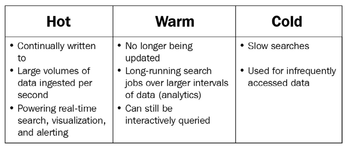
Figure 3.10 – Node data tiers in Elasticsearch
Data can be moved across the different data tiers throughout the life cycle of an index.
Ingest nodes
Ingest nodes run any ingest pipelines associated with an indexing request. Ingest pipelines contain processors that can transform incoming documents before they are indexed and stored on data nodes.
Ingest nodes can be run on the same host as the data nodes if an ETL tool such as Logstash is used and the transformations using ingest pipelines are minimal. Dedicated ingest nodes can be used if resource-intensive ingest pipelines are required.
Coordinator nodes
All Elasticsearch nodes perform the coordination role by default. Coordinator nodes can route search/indexing requests to the appropriate data node and combine search results from multiple shards before returning them to the client.
Given that the coordinator role is fairly lightweight and all the nodes in the cluster must perform this role in some capacity, having dedicated coordinator nodes is generally not recommended. Performance bottlenecks on ingestion and search can usually be alleviated by adding more data nodes or ingest nodes (if utilizing heavy ingest pipelines), rather than using dedicated coordinator nodes.
Machine learning nodes
Machine learning nodes run machine learning jobs and handle machine learning-related API requests. Machine learning jobs can be fairly resource-intensive (mostly CPU-bound since models have memory limits) and can benefit from running on a dedicated node.
Machine learning jobs may generate resource-intensive search requests on data nodes when feeding input to models. Additional machine learning nodes can be added to scale the capacity for running jobs as required, while data nodes need to be scaled to alleviate load from ML input operations.
Note
Machine learning is a paid subscription feature. A trial license can be enabled if you wish to learn and test machine learning functionality.
Elasticsearch clusters
A group of Elasticsearch nodes can form an Elasticsearch cluster. When a node starts up, it initiates the cluster formation process by trying to discover the master-eligible nodes. A list of master-eligible nodes from previous cluster state information is gathered if available. The seed hosts that have been configured on the node are also added to this list before they are checked for a master-eligible node. If a master-eligible node is found, it is sent a list of all other discovered master-eligible nodes. The newly discovered node, in turn, sends a list of all nodes it knows about. This process is repeated for all the nodes in the cluster. All the nodes in a cluster should have the same cluster.name attribute to join and participate in a cluster.
Once sufficient master-eligible nodes have been discovered to form a quorum, an election process selects the active master node, which can then make decisions on cluster state and changes.
Searching for data
Now that we understand some of the core aspects of Elasticsearch (shards, indices, index mappings/settings, nodes, and more), let's put it all together by ingesting a sample dataset and searching for data.
Indexing sample logs
Follow these steps to ingest some Apache web access logs into Elasticsearch:
- Navigate to the Chapter3/searching-for-data directory in the code repository for this book. Inspect the web.log file to see the raw data that we are going to load into Elasticsearch for querying:
head web.log
- A Bash script called load.sh has been provided for loading two items into your Elasticsearch cluster:
(a) An index template called web-logs-template that defines the index mappings and settings that are compliant with the Elastic Common Schema:
cat web-logs-template.json
(b) An ingest pipeline called web-logs-pipeline that parses and transforms logs from your dataset into the Elastic Common Schema:
cat web-logs-pipeline.json
Ingest pipelines will be covered in more detail in Chapter 4, Leveraging Insights and Managing Data on Elasticsearch.
- Run load.sh to load the components previously mentioned. Enter your Elasticsearch cluster URL. Use the elastic username and password if security has been set up on your cluster. Leave it blank if your cluster does not require authentication:
./load.sh
If successful, the script should return a response, as shown in the following screenshot:

Figure 3.11 – Components successfully loaded into Elasticsearch
- Download the Logstash .tar archive from https://www.elastic.co/downloads/logstash for your platform. The archive can be downloaded on the command line as follows:
wget https://artifacts.elastic.co/downloads/logstash/
logstash-8.0.0-darwin-x86_64.tar.gz
Uncompress and extract the files from the .tar archive once downloaded:
tar -xzf logstash-8.0.0-darwin-x86_64.tar.gz
- Edit the web-logs-logstash.conf Logstash pipeline to update the Elasticsearch host, user, and password parameters so that you can connect (and authenticate) to your cluster.
The configuration file should look as follows:

Figure 3.12 – Logstash pipeline configuration file
The Logstash pipeline accepts events using standard input and sends them to Elasticsearch for indexing. In this instance, messages are parsed and transformed using an ingest pipeline on Elasticsearch (configured by the pipeline parameter). We will look at making similar transformations using Logstash in Chapter 7, Using Logstash to Extract, Transform, and Load Data.
The Logstash executable is available in the /usr/share/logstash directory on Linux environments, when installed using the Debian or RPM package:
/usr/share/bin/logstash -f web-logs-logstash.conf < web.log
- Confirm that the data is available on Elasticsearch:
GET web-logs/_count
GET web-logs/_search
The web-logs index should contain about 20,730 documents, as shown in the following screenshot:

Figure 3.13 – Number of documents and hits in the web-logs index
The index now contains sample data for testing different types of search queries.
Running queries on your data
Data on indices can be searched using the _search API. Search requests can be run on one or more indices that match an index pattern (as in the case of index templates).
Elasticsearch queries are described using Query DSL. The reference guide contains an exhaustive list of supported query methods and options:
https://www.elastic.co/guide/en/elasticsearch/reference/8.0/query-dsl.html
In this section, we will look at some basic questions we want to ask about our data and how we can structure our queries to do so:
- Find all the HTTP events with an HTTP response code of 200.
A term query can be used on the http.response.status_code field, as shown in the following request:
GET web-logs/_search
{
"query": {
"term": {
"http.response.status_code": { "value": "200" }
}
}
}
The query should return a large number of hits (more than 10,000), as shown in the following screenshot:

Figure 3.14 – Hits for HTTP 200 events
- Find all HTTP events where the request method was of the POST type and resulted in a non-200 response code.
Use two term queries within a bool compound query. The must and must_not clauses can be used to exclude all 200 response codes, as shown in the following request:
GET web-logs/_search
{
"query": {
"bool": {
"must_not": [
{ "term": {
"http.response.status_code": { "value": "200" }
}
],
"must": [
{ "term": {
"http.request.method": { "value": "POST" }
}
}
]
}
}
}
The query should return 22 hits, as follows:

Figure 3.15 – Hits for unsuccessful HTTP POST events
A match query can be used on the event.original field. The and operator requires that both words (tokens) exist in the resulting document. Run the following query:
GET web-logs/_search
{
"query": {
"match": {
"event.original":{
"query": "refrigerator windows",
"operator": "and"
}
}
}
}
- Look for all requests where users on Windows machines were looking at refrigerator-related pages on the website.
Use a bool compound query with two match queries, as shown in the following command block:
GET web-logs/_search
{
"query": {
"bool": {
"must": [
{ "match": { "url.original.text": "refrigerator" }},
{ "match": { "user_agent.os.full.text": "windows" }}
]
}
}
}
The query should return four hits, as follows:

Figure 3.16 – Hits for Windows users looking for refrigerators
Use a terms match query to look for the existence of a term in the list of terms, as shown in the following command block:
GET web-logs/_search
{
"query": {
"terms": {
"source.geo.country_name": [
"South Africa",
"Ireland",
"Hong Kong"
]
}
}
}
- Find all the events originating from IP addresses belonging to the Pars Online PJS and Respina Networks & Beyond PJSC telecommunication providers.
Create an index where you can store a list of telecommunications providers. This is an alternative to defining the providers as part of a query, making it a useful option when a large list of terms needs to be searched:
PUT telcos-list
{
"mappings": {
"properties": { "name": { "type": "keyword" }}
}
}
Index a document containing the list of terms to be searched:
PUT telcos-list/_doc/1
{
"name": ["Pars Online PJS", "Respina Networks & Beyond PJSC"]
}
Use a terms query with an index lookup to find the hits:
GET web-logs/_search
{
"query": {
"terms": {
"source.as.organization.name": {
"index" : "telcos-list",
"id" : "1",
"path" : "name"
}
}
}
}
The query should return 1,538 hits, as shown in the following screenshot:

Figure 3.17 – All requests originating from a group of telecommunications providers
- Find all HTTP GET events with response bodies of more than 100,000 bytes.
Use a bool query containing a term match for GET events and a range filter for the numeric http.response.body.bytes field, as shown here:
GET web-logs/_search
{
"query": {
"bool": {
"must": [
{ "term": { "http.request.method": { "value": "GET" }}},
{ "range": { "http.response.body.bytes": { "gte": 100000 }}}
]
}
}
}
Inspect the results to confirm that the hits meet the parameters of our search.
Summary
In this chapter, we briefly looked at three core aspects of Elasticsearch.
First, we looked at the internals of an index in Elasticsearch. We explored how settings can be applied to indices and learned how to configure mappings for document fields. We also looked at a range of different data types that are supported and how they can be leveraged for various use cases.
We then looked at how nodes on Elasticsearch host indices and data. We understood the different roles a node plays as part of a cluster, as well as the concept of data tiers, to take advantage of different hardware profiles on nodes, depending on how the data is used.
Lastly, we ingested some sample data and learned how to ask questions about our data using the search API.
In the next chapter, we will dive a little bit deeper into how to derive statistical insights, use ingest pipelines to transform data, create entity-centric indices by pivoting on incoming data, manage time series sources using life cycle policies, back up data into snapshots. and set up real-time alerts.