Chapter 8: Jumpstarting ML with SageMaker JumpStart and Autopilot

SageMaker JumpStart offers complete solutions for select use cases as a starter kit for the world of machine learning (ML) with Amazon SageMaker without any code development. SageMaker JumpStart also catalogs popular pretrained computer vision (CV) and natural language processing (NLP) models for you to easily deploy or fine-tune for your dataset. SageMaker Autopilot is an AutoML solution that explores your data, engineers features on your behalf, and trains an optimal model from various algorithms and hyperparameters. You don't have to write any code: Autopilot does it for you and returns notebooks to show you how it does it.

In this chapter, we will cover the following topics:

• Launching a SageMaker JumpStart solution
• Deploying and fine-tuning a model from the SageMaker JumpStart model zoo
• Creating a high-quality model with SageMaker Autopilot

Technical requirements

For this chapter, you need to have permission to use JumpStart templates. You can confirm it from your domain and user profile. The code used in this chapter can be found at https://github.com/PacktPublishing/Getting-Started-with-Amazon-SageMaker-Studio/tree/main/chapter08.

Launching a SageMaker JumpStart solution

SageMaker JumpStart is particularly useful if you would like to learn a set of best practices for how AWS services should be used together to create an ML solution. You can do the same, too. Let's open up the JumpStart browser. There are multiple ways to open it, as shown in Figure 8.1. You can open it from the SageMaker Studio Launcher on the right or from the JumpStart asset browser in the left sidebar.

Figure 8.1 – Opening the JumpStart browser from the Launcher or the left sidebar

A new tab named SageMaker JumpStart will pop up in the main working area. Go to the Solutions section and click View all, as shown in Figure 8.2.

Figure 8.2 – Viewing all solutions in JumpStart

Let's next move on to the solutions catalog for industries.

Solution catalog for industries

There are more than a dozen solutions available in JumpStart as shown in Figure 8.3. These solutions are based on use cases spanning multiple industries, including manufacturing, retail, and finance.

Figure 8.3 – JumpStart solution catalog – Click each card to see more information

They are created by AWS developers and architects who know the given industry and use case. You can read more about each use case by clicking on the card. You will be greeted with a welcome page describing the use case, methodology, dataset, solution architecture, and any other external resources. On each solution page, you should also see a Launch button, which will deploy the solution and all cloud resources into your AWS account from a CloudFormation template.

Let's use the Product Defect Detection solution from the catalog as our example, and we will walk through the deployment and the notebooks together.

Deploying the Product Defect Detection solution

Visual inspection is widely adopted as a quality control measure in manufacturing processes. Quality control used to be a manual process where staff members would visually inspect the product either on the line or via imagery captured with cameras. However, manual inspection does not scale for the large quantities of products created in factories today. ML is a powerful tool that can identify product defects at an error rate that may, if trained properly, be even better than a human inspector. The Product Defect Detection SageMaker JumpStart solution is a great starting point to jump-start your CV project to detect defects in images using a state-of-the-art deep learning model. You will see how SageMaker manages training with a PyTorch script, and how model hosting is used. You will also learn how to make inferences against a hosted endpoint. The dataset is a balanced dataset across six types of surface defects and contains ground truths for both classification and drawing bounding boxes. Please follow these steps and read through the content of the notebooks:

1. From the Solution catalog, please select Product Defect Detection in Images. As shown in Figure 8.4, you can read about the solution on the main page. You can learn about the sample data, the algorithm, and the cloud solution architecture.

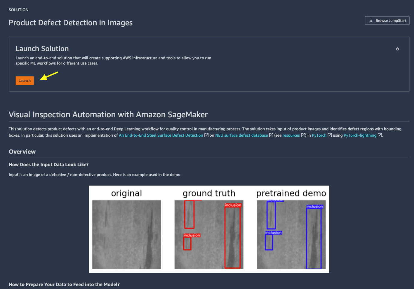
Figure 8.4 – Main page of the Product Defect Detection in Images solution

2. Hit the Launch button, as shown in Figure 8.4, to start the deployment. You should see the deployment in progress on the screen. What is happening is that we just initiated a resource deployment using AWS CloudFormation in the background. AWS CloudFormation is a service that helps create, provision, and manage AWS resources in an orderly fashion through a template in JSON or YAML declarative code. This deployment takes a couple of minutes.
3. Once the solution becomes Ready, click on Open Notebook in the tab to open the first notebook, 0_demo.ipynb, from the solution. This notebook is the first of four notebooks that are deployed as part of the CloudFormation setup into your home directory at S3Downloads/jumpstart-prod-dfd_xxxxxxx/notebooks/. The notebook requires the SageMaker JumpStart PyTorch 1.0 kernel as we are going to build a PyTorch-based solution. The kernel startup might take a minute or two if this is the first time using the kernel.
4. Run all the cells in the 0_demo.ipynb notebook. This notebook downloads the NEU-DET detection dataset to the filesystem and creates a SageMaker hosted endpoint using the SageMaker SDK's sagemaker.pytorch.PyTorchModel class for a pretrained PyTorch model. At the end of the notebook, you should see a figure showing the patches detected by the pretrained model compared to the ground truth, as in Figure 8.5.

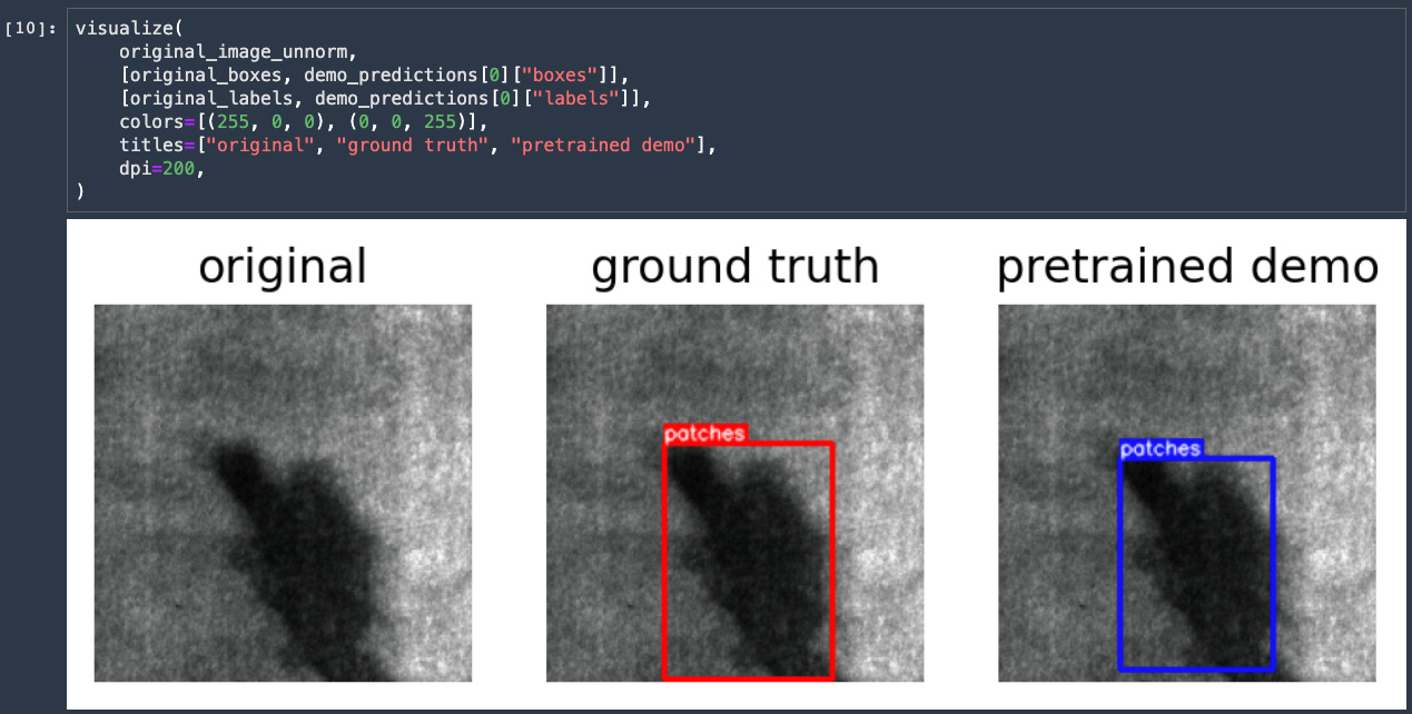
Figure 8.5 – Final output of the 0_demo.ipynb notebook, showing a steel surface example, the ground truth, and the model prediction by a pretrained model

This notebook demonstrates a key flexibility SageMaker offers, that is, you can bring a model trained from outside of SageMaker and host it in SageMaker. To create a SageMaker model from a PyTorch model, you need the model file .pt/.pth archived in a model.tar.gz archive and an entry point, detector.py script in this case, that instructs how the inference should be made. We can take a look at the detector.py script to learn more.

5. (Optional) Add a new cell and fill in the following commands:

   !aws s3 cp {sources}source_dir.tar.gz .

   !tar zxvf source_dir.tar.gz

This will get the entire code base locally. Please open the detector.py file and locate the part that SageMaker uses to make inferences:

def model_fn(model_dir):

    backbone = "resnet34"

    num_classes = 7  # including the background

    mfn = load_checkpoint(Classification(backbone, num_classes - 1).mfn, model_dir, "mfn")

    rpn = load_checkpoint(RPN(), model_dir, "rpn")

    roi = load_checkpoint(RoI(num_classes), model_dir, "roi")

    model = Detection(mfn, rpn, roi)

    model = model.eval()

    freeze(model)

    return model

SageMaker requires at least a model_fn(model_dir) function when importing a PyTorch model to instruct how the model is defined. In this example, Detection()class is a GeneralizedRCNN model defined in S3Downloads/jumpstart-prod-dfd_xxxxxx/notebooks/sagemaker_defect_detection/models/ddn.py with weights loaded from the provided model.

Note

Other inference related functions you can implement include the following:

Deserializing the invoke request body into an object we can perform prediction on:

input_object = input_fn(request_body, request_content_type)

Performing prediction on the deserialized object with the loaded model:

prediction = predict_fn(input_object, model)

Serializing the prediction result into the desired response content type:

output = output_fn(prediction, response_content_type)

SageMaker has default implementations for these three functions if you don't override them. If you have a custom approach for making inferences, you can override these functions.

6. Proceed to the end of the notebook and click on Click here to continue to advance to the next notebook, 1_retrain_from_checkpoint.ipynb.
7. Run all the cells in 1_retrain_from_checkpoint.ipynb. This notebook fine-tunes the pretrained model from a checkpoint with the downloaded dataset for a few more epochs. The solution includes training code in detector.py from osp.join(sources, "source_dir.tar.gz"). The solution uses the SageMaker SDK's PyTorch estimator to create a training job that launches an on-demand compute resource of one ml.g4dn.2xlarge instance and trains it from a provided pretrained checkpoint. The training takes about 10 minutes. The following lines of code show how you can feed the training data and a pretrained checkpoint to SageMaker PyTorch estimator to perform a model fine-tuning job:

   finetuned_model.fit(

       {

           "training": neu_det_prepared_s3,

           "pretrained_checkpoint": osp.join(s3_pretrained, "epoch=294-loss=0.654-main_score=0.349.ckpt"),

       }

   )

   Note

   The naming of the dictionary keys to .fit() call is done by design. These keys are registered as environment variables with a SM_CHANNEL_ prefix inside the training container and can be accessed in the training script. The keys need to match what is written in the detector.py file in order to make this .fit() training call work. For example, see line 310 and 349 in detector.py:

   aa("--data-path", metavar="DIR", type=str, default=os.environ["SM_CHANNEL_TRAINING"])

   aa("--resume-sagemaker-from-checkpoint", type=str, default=os.getenv("SM_CHANNEL_PRETRAINED_CHECKPOINT", None))

After the training, the model is deployed as a SageMaker hosted endpoint, as in the 0_demo.ipynb notebook. In the end, a comparison between the ground truth, the inference from the pretrained model from 0_demo.ipynb, and the inference from the fine-tuned model is visualized. We can see that the inference from the fine-tuned model has one fewer false positive, yet still isn't able to pick up a patch on the right side of the sample image. This should be considered a false negative.

8. Proceed to click on Click here to continue to advance to the next notebook, 2_detection_from_scratch.ipynb.
9. Run all the cells in the 2_detection_from_scratch.ipynb notebook. Instead of training from a checkpoint, we train a model from scratch with 10 epochs using the same dataset and compare the inference to that from the pretrained model. The model is significantly undertrained, as expected with the small epoch size used. You are encouraged to increase the epoch size (the EPOCHS variable) to 300 to achieve better performance. However, this will take significantly more than 10 minutes.

   Note

   We control whether we train from a checkpoint or from scratch by whether we include a pretrained_checkpoint key in a dictionary to .fit() or not.

10. Proceed to click on Click here to continue to advance to the next notebook, 3_classification_from_scratch.ipynb.

In this notebook, we train a classification model using classifier.py for 50 epochs, instead of an object detection model from scratch, using the NEU-CLS classification dataset. A classification model is different from the previous object detection models. Image classification recognizes the types of defect in an entire image, whereas an object detection model can also localize where the defect is. Image classification is useful if you do not need to know the location of the defect, and can be used as a triage model for product defects.

Training a classification model is faster, as you can see from the job. The classification accuracy on the validation set reaches 0.99, as shown in the cell output from the training job, which is very accurate:

Epoch 00016: val_acc reached 0.99219 (best 0.99219), saving model to /opt/ml/model/epoch=16-val_loss=0.028-val_acc=0.992.ckpt as top 1

11. This is the end of the solution. Please make sure to execute the last cell in each notebook to delete the models and endpoints, especially the last cell in the 0_demo.ipynb notebook, where the deletion is commented out. Please uncomment this and execute it to delete the pretrained model and endpoint.

With this SageMaker JumpStart solution, you built and trained four deep learning models based on a PyTorch implementation of Faster RCNN to detect and classify six types of defects in steel imagery with minimal coding effort. You also hosted them as SageMaker endpoints for real-time prediction. You can expect a similar experience with other solutions in SageMaker JumpStart to learn different aspects of SageMaker features used in the context of solving common use cases.

Now, let's switch gears to the SageMaker JumpStart model zoo.

SageMaker JumpStart model zoo

There are more than 200 popular prebuilt and pretrained models in SageMaker JumpStart for you to use out of the box or continue to train for your use case. What are they good for? Training an accurate deep learning model is time consuming and complex, even with the most powerful GPU machine. It also requires large amounts of training and labeled data. Now, with these models that have been developed by the community, pretrained on large datasets, you do not have to reinvent the wheel.

Model collection

There are two groups of models: text models and vision models in SageMaker JumpStart model zoo. These models are the most popular ones among the ML community. You can quickly browse the models in SageMaker JumpStart and select the one that meets your needs. On each model page, you will see an introduction to the model, its usage, and how to prepare a dataset for fine-tuning purposes. You can deploy models into AWS as a hosted endpoint for your use case or fine-tune the model further with your own dataset.

Text models are sourced from the following three hubs: TensorFlow Hub, PyTorch Hub, and Hugging Face. Each model is specifically trained for a particular type of NLP task using a dataset such as text classification, question answering, or text generation. Notably, there are many flavors of Bidirectional Encoder Representations from Transformers (BERT), Cross-lingual Language Model (XLM), ELECTRA, and Generative Pretrained Transformer (GPT) up for grabs.

Vision models are sourced from TensorFlow Hub, PyTorch Hub, and Gluon CV. There are models that perform image classification, image feature vector extraction, and object detection. Inception, SSD, ResNet, and Faster R-CNN models are some of the most notable and widely used models in the field of CV.

Deploying a model

Let's find a question-answering model and see how we can deploy it to our AWS account. In the search bar, type in question answering hit Return, and you should see a list of models that perform such tasks returned to you, as shown in Figure 8.6.

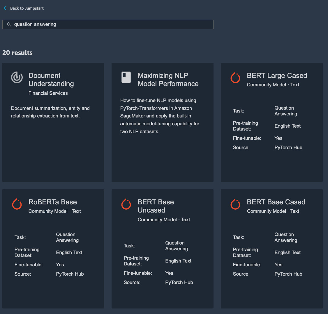
Figure 8.6 – Searching for question-answering models

Let's find and double-click DistilRoBERTa Base for Question Answering in the search results. This model is trained on OpenWebTextCorpus and is distilled from the RoBERTa model checkpoint. It has 6 layers, 768 hidden, 12 heads, and 82 million parameters. 82 million! It is not easy to train such a large model, for sure. Luckily with SageMaker JumpStart, we have a model that we can deploy out of the box. As shown in Figure 8.7, please expand the Deployment Configuration section, choose Ml.M5.Xlarge as the machine type, leave the endpoint name as default, and hit Deploy. Ml.M5.Xlarge is a general-purpose instance type that has 4 vCPU and 16 GB of memory, which is sufficient for this example. The deployment will take a couple of minutes.

Figure 8.7 – Deploying a JumpStart DistilRoBERTa Base model

Once the model is deployed, a notebook will be provided to you to show how you can make an API call to the hosted endpoint (Figure 8.8). You can find a list of models in the JumpStart left sidebar.

Figure 8.8 – Opening a sample inference notebook after the model is deployed

In the sample notebook, two questions from the SQuAD v2 dataset, one of the most widely used question-answering datasets for evaluation, are provided to show how inferencing can be done. Let's also ask our model other questions based on the following passage (Can you guess where you've read it before? Yes, it's the opening statement of this chapter!):

Context:

SageMaker JumpStart offers complete solutions for select use cases as a starter kit to the world of machine learning (ML) with Amazon SageMaker without any code development. SageMaker JumpStart also catalogs popular pretrained computer vision (CV) and natural language processing (NLP) models for you to easily deploy or fine-tune to your dataset. SageMaker Autopilot is an AutoML solution that explores your data, engineers features on your behalf, and trains an optimal model from various algorithms and hyperparameters. You don't have to write any code: Autopilot does it for you and returns notebooks to show how it does it.

Questions:

• What does SageMaker JumpStart do?
• What is NLP?

In the notebook, we should add the following to the second cell:

question_context3 = ["What does SageMaker JumpStart do?", "SageMaker JumpStart offers complete solutions for select use cases as a starter kit to the world of machine learning (ML) with Amazon SageMaker without any code development. SageMaker JumpStart also catalogs popular pretrained computer vision (CV) and natural language processing (NLP) models for you to easily deploy or fine-tune to your dataset. SageMaker Autopilot is an AutoML solution that explores your data, engineers features on your behalf and trains an optimal model from various algorithms and hyperparameters. You don't have to write any code: Autopilot does it for you and returns notebooks to show how it does it."]

question_context4 = ["What is NLP?", question_context3[-1]]

In the third cell, append the two new question context pairs to the list in the for loop and execute all cells in the notebook:

for question_context in [question_context1, question_context2, question_context3, question_context4]:

And voila! We get responses from our model that answer our questions about SageMaker JumpStart's capabilities and the full form of NLP as natural language processing.

Fine-tuning a model

It is typical to perform model fine-tuning when you take a pretrained model off the shelf to expose the model to your dataset so that it can perform better on your dataset compared to the performance without such exposure. Furthermore, model fine-tuning takes less training time and requires a smaller amount of labeled data compared to training a model from scratch. To fine-tune a pretrained model from SageMaker JumpStart, first we need to make sure that the model you would like to use supports fine-tuning. You can find this attribute in the overview cards. Secondly, you need to point a dataset to the model. Taking the DistilRoBERTa Base model as an example, SageMaker JumpStart provides the default dataset of SQuAD-v2, which allows you to quickly start a training job. You can also create a dataset of your own by following the instructions on the JumpStart model page. We are going to do just that.

Let's fine-tune the base DistilRoBERTa Base model with some questions and answers about Buddhism, which is one of the topics in the SquAD-v2 dataset. Please follow these steps:

1. Open the chapter08/1-prep_data_for_finetune.ipynb notebook in the repository and execute all cells to download the dataset, extract the paragraphs that are related to Buddhism, and organize them as the fine-tune trainer expects. This is detailed on the description page in the Fine-tune the Model on a New Dataset section:
   • Input: A directory containing a data.csv file:
     • The first column of the data.csv should have a question.
     • The second column should have the corresponding context.
     • The third column should have the integer character starting position for the answer in the context.
     • The fourth column should have the integer character ending position for the answer in the context.
   • Output: A trained model that can be deployed for inference.
2. At the end of the notebook, the data.csv file will be uploaded to your SageMaker default bucket: s3://sagemaker-<region>-<accountID>/chapter08/buddhism/data.csv.
3. Once this is done, let's switch back to the model page and configure the fine-tuning job. As in Figure 8.9, select Enter S3 bucket location, paste in your CSV file URI into the box below, optionally append -buddhism onto the model name, leave the machine type and hyperparameters as their defaults, and hit Train. The default Ml.P3.2xlarge instance type, with one NVIDIA Tesla V100 GPU, is a great choice for fast model fine-tuning. The default hyperparameter setting performs fine-tuning with a batch size of 4, learning rate of 2e-5, and 3 epochs. This is sufficient for us to demonstrate how the fine-tuning works. Feel free to change the values here to reflect your actual use case.

Figure 8.9 – Configuring a fine-tuning job for a custom dataset

The training job should take about 6 minutes with the Ml.P3.2xlarge instance.

4. Once the job completes, you can deploy the model to an endpoint with an Ml.M5.Xlarge instance, as shown in Figure 8.10. Ml.M5.Xlarge is a general-purpose CPU instance, which is a good starting point for model hosting.

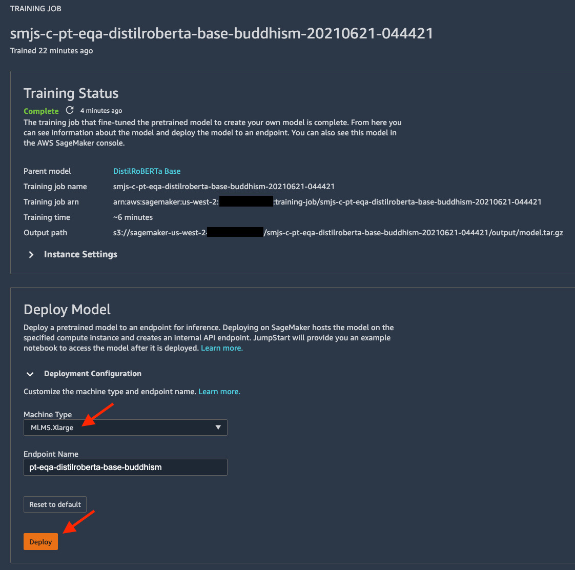
Figure 8.10 – Deploying the fine-tuned model

Of course, we now need to test how well the fine-tuned model performs on questions related to Buddha and Buddhism. Once the deployment finishes, you will be prompted with an option to open a prebuilt notebook to use the endpoint, similar to what is shown in Figure 8.8.

5. We can replace the question-context pair in the second cell with the following snippet from https://www.history.com/topics/religion/buddhism:

   question_context1 = ["When was Buddhism founded?", "Buddhism is a faith that was founded by Siddhartha Gautama ("the Buddha") more than 2,500 years ago in India. With about 470 million followers, scholars consider Buddhism one of the major world religions. Its practice has historically been most prominent in East and Southeast Asia, but its influence is growing in the West. Many Buddhist ideas and philosophies overlap with those of other faiths."]

   question_context2 = ["Where is Buddhism popular among?", question_context1[-1]]

Then, execute the cells in the notebook and you will see how well our new model performs.

It's not quite what we would like the model to be. This is due to the very small epochs used and perhaps the unoptimized batch size and learning rate. As we are providing new data points for the model, the weights in the network are once again being updated and need to perform training for a sufficient number of epochs to converge on a lower loss and thus create a more accurate model. These hyperparameters often need to be tuned in order to obtain a good model even with fine-tuning. You are encouraged to further experiment with different hyperparameters to see if the model provides better responses to the questions.

We have just created three ML models, which are supposed to be complex and difficult to train, without much coding at all. Now we are going to learn how to use SageMaker Autopilot to automatically create a high-quality model without any code.

Creating a high-quality model with SageMaker Autopilot

Have you ever wanted to build an ML model without the hassle of data preprocessing, feature engineering, exploring algorithms, and optimizing the hyperparameters? Have you ever thought about how, for some use cases, you just wanted something quick to see if ML is even a possible approach for a certain business use case? Amazon SageMaker Autopilot makes it easy for you to build an ML model for tabular datasets without any code.

Wine quality prediction

To demonstrate SageMaker Autopilot, let's use a wine quality prediction use case. The wine industry has been searching for a technology that can help winemakers and the market to assess the quality of wine faster and with a better standard. Wine quality assessment and certification is a key part of the wine market in terms of production and sales and prevents the illegal adulteration of wines. Wine assessment is performed by expert oenologists based on physicochemical and sensory tests that produce features such as density, alcohol level, and pH level. However, when a human is involved, the standard can vary between oenologists or between testing trials. Having an ML approach to support oenologists in providing analytical information therefore becomes an important task in the wine industry.

We are going to train an ML model to predict wine quality based on the physicochemical sensory values for 4,898 white wines produced between 2004 and 2007 in Portugal. The dataset is available from UCI at https://archive.ics.uci.edu/ml/datasets/Wine+Quality.

Setting up an Autopilot job

Let's begin:

1. Please open the chapter08/2-prep_data_for_sm_autopilot.ipynb notebook from the repository, and execute all of the cells to download the data from the source, hold out a test set, and upload the training data to an S3 bucket. Please note the paths to the training data.
2. Next, open the Launcher and select New Autopilot Experiment, as in Figure 8.11.

Figure 8.11 – Creating a new Autopilot experiment

A new window will pop up for us to configure an Autopilot job.

3. As shown in Figure 8.12, provide an Experiment name of your choice, such as white-wine-predict-quality.

Figure 8.12 – Configuring an Autopilot job

4. As shown in Figure 8.12, provide the training data in the CONNECT YOUR DATA section, check the Find S3 bucket radio button, select your sagemaker-<region>-<accountID> from the S3 bucket name drop-down menu, and select the sagemaker-studio-book/chapter08/winequality/winequality-white-train.csv file from the Dataset file name drop-down menu. Set Target to quality to predict the quality of wine with the rest of attributes in the CSV file.
5. In the lower half of the configuration page, as shown in Figure 8.13, provide a path to save the output data to, check the Find S3 bucket radio button, select your sagemaker-<region>-<accountID> from the S3 bucket name drop-down menu, and paste the sagemaker-studio-book/chapter08/winequality/ path into the Dataset directory name field as the output location. This path is where we have the training CSV file.

Figure 8.13 – Configuring an Autopilot job

6. As shown in Figure 8.13, choose Multiclass classification from the Select the machine learning problem type drop-down menu. Then choose F1macro from the Objective metric drop-down menu so that we can expect a more balanced model should the data be biased toward a certain quality rank.
7. As shown in Figure 8.13, choose Yes for Do you want to run a complete experiment?. Then toggle the Auto deploy option to off as we would like to walk through the evaluation process in SageMaker Studio before deploying our best model.
8. As shown in Figure 8.13, expand the ADVANCED SETTINGS – Optional section and input 100 in the Max candidates field. By default, Autopilot runs 250 training jobs with different preprocessing steps, training algorithms, and hyperparameters. By using a limited number of candidates, we should expect the full experiment to complete faster than with the default setting.
9. Hit Create Experiment to start the Autopilot job.

You will see a new window that shows the progress of the Autopilot job. Please let it crunch the numbers a bit and come back in a couple of minutes. You will see more progress and output in the progress tab, as shown in Figure 8.14.

Figure 8.14 – Viewing the progress of an Autopilot experiment

A lot is going on here. Let's dive in.

Understanding an Autopilot job

Amazon SageMaker Autopilot executes an end-to-end ML model-building exercise automatically. It performs exploratory data analysis (EDA), does data preprocessing, and creates feature engineering and a model-training recipe. It then executes the recipe in order to find the best model given the conditions. You can see the progress in the middle portion of Figure 8.14.

What makes Autopilot unique is the full visibility that it provides. Autopilot unboxes the typical AutoML black box by giving you the EDA results and the code that Autopilot runs to perform the feature engineering and ML modeling in the form of Jupyter notebooks. You can access the two notebooks by clicking the Open data exploration notebook button for the EDA results and the Open candidate generation notebook button for the recipe.

The data exploration notebook is helpful for understanding the data, the distribution, and how Autopilot builds the recipe based on the characteristics of the data. For example, Autopilot looks for missing values in the dataset, the distribution of numerical features, and the cardinality of the categorical features. This information gives data scientists a baseline understanding of the data, along with actionable insights on whether the input data contains reasonable entries or not. Should you see many features with high percentages of missing values (the Percent of Missing Values section), you could take the suggested actions to investigate the issue from the data creation perspective and apply some level of pre-processing to either remove the feature or apply domain-specific imputation. You may ask, "Doesn't Autopilot apply data pre-processing and feature engineering to the data?" Yes, it does. However, Autopilot does not have domain-specific knowledge of your data. You should expect a more generic, data science-oriented approach to the issues surfaced by Autopilot, which may not be as effective.

The candidate generation notebook prescribes a recipe for how the model should be built and trained based on the EDA of the data. The amount of code might look daunting, but if you read through it carefully, you can see, for example, what data preprocessing steps and modeling approaches Autopilot is attempting, as shown in the Candidate Pipelines section. The following is one example of this:

The SageMaker Autopilot Job has analyzed the dataset and has generated 9 machine learning pipeline(s) that use 3 algorithm(s).

Autopilot bases the pipelines on three algorithms: XGBoost, linear learner, and multi-layer perceptron (MLP). XGBoost is a popular gradient-boosted tree algorithm that combines an ensemble of weak predictors to form the final predictor in an efficient and flexible manner. XGBoost is one of SageMaker's built-in algorithms. Linear learner, also a SageMaker built-in algorithm, trains multiple linear models with different hyperparameters, and finds the best model with a distributed stochastic gradient descent optimization. MLP is a neural network-based supervised learning algorithm that can have multiple hidden layers of neurons to create a non-linear model.

You can also see the list of hyperparameters and ranges Autopilot is exploring (the MultiAlgorithm Hyperparameter Tuning section). Not only does Autopilot provide you visibility, but it also gives you full control of the experimentation. You can click on the Import notebook button the top right to get a copy of the notebook that you can actually customize and execute to obtain your next best model.

Evaluating Autopilot models

If you see that the job status in the tab, as shown in Figure 8.14, has changed to Completed, then it is time to evaluate the models Autopilot has generated. Autopilot has trained 100 models using various mixtures of feature engineering, algorithms, and hyperparameters as you can see in the list of trials. This leaderboard also shows the performance metric, the F1 score on a random validation split, used to evaluate the models. You can click on Objective: F1 to sort the models by score.

Let's take a closer look at the best model, the one that has the highest F1 score and a star next to the trial name. Right-click on the trial and select Open in model details to view more information.

Figure 8.15 – Viewing Autopilot model details in SageMaker Studio

Autopilot reports a lot of detail on this page, as shown in Figure 8.15. First of all, we can see that this model is built based on the XGBoost algorithm. We also see a chart of feature importance that Autopilot generates for our convenience. This chart tells us how the model considers the importance, or contribution, of the input features. Autopilot computes the SHapley Additive exPlanations (SHAP) values using SageMaker Clarify for this XGBoost model and dataset. SHAP values explain how features contribute to the model forming the decision based on game theory.

Note

You can hover over the bars to see the actual values. SageMaker provides more detail so that you can learn more about how these SHAP values are calculated in the white papers in the Want to learn more? section.

Back to the chart, you can also download an automatically generated PDF report that contains this chart for review and distribution (Export PDF report). If you want to work with the raw data in JSON format in order to integrate the SHAP values in other applications, you can download the data (Download raw data). By clicking the two buttons, you will be redirected to the S3 console as shown in Figure 8.16. You can download the file from the S3 bucket on the console by clicking the Download button.

Figure 8.16 – Downloading the feature importance PDF report in the S3 console

Besides the feature importance, the model performance on the training and validation sets is also very important in understanding how the model would perform in real life. You can see the metrics captured during the training run in the Metrics part. In addition to the ObjectiveMetric used to rank the models on the leaderboard, we see the following metrics:

• train:f1
• train:merror
• validation:f1
• validation:merror

They are the multi-class F1macro and the multi-class error for the train and validation split of the data. As you can tell by the identical values, ObjectiveMetric is essentially validation:f1. With train:f1 well above validation:f1, we may come to the conclusion that the model is overfitted to the training dataset. But why is this?

We can further verify the model performance in more detail with the test data that we held out at the beginning. Please open the chapter08/3-evaluate_autopilot_models.ipynb notebook from the repository and execute all cells. In this notebook, you will retrieve the top models based on the ObjectiveMetric from the Autopilot job, perform inference in the cloud using the SageMaker Batch Transform feature, and run some evaluations for each model. Feel free to change the value in TOP_N_CANDIDATES to a different number. You should see the F1 score computed with the macro, an unweighted mean, weighted approaches, a classification report (from a sklearn function), and a confusion matrix on the test data as the output of the last cell.

With the top model, a couple of things jump out at me here. The data is imbalanced in nature. There is a higher concentration of scores 5, 6, and 7. Few wines got a score of 3, 4, or 8. The confusion matrix also shows that wines that got a score of 3 were all incorrectly classified. Under this situation, the f1 macro measure will be drastically lowered by incorrect classification of a minority class out of proportion. If we look at the weighted version of the f1 score, we get a significantly higher score as the scoring weights the dominant classes more heavily:

Candidate name:  white-wine-predict-qualitysZ1CBE-003-1a47413b

Objective metric name:  validation:f1

Objective metric value:  0.4073199927806854

f1 = 0.51, Precision = 0.59 (macro)

f1 = 0.67, Precision = 0.68 (weighted)

              precision    recall  f1-score   support

           3       0.00      0.00      0.00         3

           4       0.70      0.39      0.50        18

           5       0.63      0.67      0.65       144

           6       0.67      0.77      0.72       215

           7       0.76      0.57      0.65        94

           8       0.78      0.44      0.56        16

    accuracy                           0.67       490

   macro avg       0.59      0.47      0.51       490

weighted avg       0.68      0.67      0.67       490

[[  0   0   3   0   0   0]

[  0   7   8   3   0   0]

[  0   2  96  45   1   0]

[  0   1  37 166  10   1]

[  0   0   8  31  54   1]

[  0   0   0   3   6   7]]

It is also important to measure the model's performance using the metrics that matter the most to the use case. As the author of the cited study stated about the importance of precision measure:

"This statistic is important in practice, since in a real deployment setting the actual values are unknown and all predictions within a given column would be treated the same."

We should compare the precision measure used in the original research study (in Table 3 in the study, linked in the Further reading section) where the individual precisions are the following:

• 4: 63.3%
• 5: 72.6%
• 6: 60.3%
• 7: 67.8%
• 8: 85.5%

when tolerance T = 0.5 for white wines. Our first Autopilot model overperforms in precision in some categories and underperforms in others.

Another strategy to find a model that serves the business problem better is to evaluate more models in addition to the best model suggested by Autopilot. We can see the evaluation for two others (or more, depending on your setting for TOP_N_CANDIDATES). We find that even though the second and third models have lower validation:f1 (macro) scores than the first model, they actually have higher F1 scores on the held-out test set. The individual precision scores for the third model are all better than the model in the original research, except for class 5, by 2.6%. What a charm! The third model in the leaderboard actually has better performance on the test data as measured by the precision metric, which makes the most sense to the use case.

After evaluation, we can deploy the optimal model into an endpoint for real-time inference. Autopilot makes it easy to deploy a model. In the leaderboard, select the line item that you would like to deploy, and click on the Deploy model button. A new page will pop up for you to configure the endpoint. Most options are straightforward and self-explanatory for an experienced SageMaker Studio user. Two things to note are that you can enable the data capture, which is useful if you want to set up SageMaker Model Monitor later. If you want the model to return more than just the predicted_label, such as the hard label of the winning class in a multiclass use case, you can choose to return the probability of the winning label, the labels of all classes, and the probabilities of all classes. The order of the selection will also determine the order of the output.

Summary

In this chapter, we introduced two features integrated into SageMaker Studio—JumpStart and Autopilot—with three ML use cases to demonstrate low-to-no code ML options for ML developers. We learned how to browse JumpStart solutions in the catalog and how to deploy an end-to-end CV solution from JumpStart to detect defects in products. We also deployed and fine-tuned a question-answering model using the DistilRoBERTa Base model from the JumpStart model zoo without any ML coding. With Autopilot, we built a white wine quality prediction model simply by pointing Autopilot to a dataset stored in S3 and starting an Autopilot job – no code necessary. It turned out that Autopilot even outperforms the model created by the original researchers, which may have taken months of research.

With the next chapter, we begin the next part of the book: Production and Operation of Machine Learning with SageMaker Studio. We will learn how we can move from prototyping to production ML training at scale with distributed training in SageMaker, how to monitor model training easily with SageMaker Debugger, how to save training cost with managed spot training..

Further reading

For more information take a look at the following resources:

• P. Cortez, A. Cerdeira, F. Almeida, T. Matos and J. Reis. Modeling wine preferences by data mining from physicochemical properties. In Decision Support Systems, Elsevier, 47(4):547-553, 2009. https://bit.ly/3enCZUz