Chapter 10: Monitoring ML Models in Production with SageMaker Model Monitor

Having a model put into production for inferencing isn't the end of the machine learning (ML) life cycle. It is just the beginning of an important topic: how do we make sure the model is performing as it is designed to and as expected in real life? Monitoring how the model performs in production, especially on data that the model has never seen before, is made easy with SageMaker Studio. You will learn how to set up model monitoring for models deployed in SageMaker, detect data drift and performance drift, and visualize results in SageMaker Studio, so that you can let the system detect the degradation of your ML model automatically.

In this chapter, we will be learning about the following:

• Understanding drift in ML
• Monitoring data and model performance drift in SageMaker Studio
• Reviewing model monitoring results in SageMaker Studio

Technical requirements

For this chapter, you need to access the code in https://github.com/PacktPublishing/Getting-Started-with-Amazon-SageMaker-Studio/tree/main/chapter10.

Understanding drift in ML

An ML model in production needs to be carefully and continuously monitored for its performance. There is no guarantee that once the model is trained and evaluated, it will be performing at the same level in production as in the testing environment. Unlike a software application, where unit tests can be implemented to test out an application in all possible edge cases, it is rather hard to monitor and detect issues of an ML model. This is because ML models use probabilistic, statistical, and fuzzy logic to infer an outcome for each incoming data point, and the testing, meaning the model evaluation, is typically done without true prior knowledge of production data. The best a data scientist can do prior to production is to create training data from a sample that closely represents the real-world data, and evaluate the model with an out-of-sample strategy in order to get an unbiased idea of how the model would perform on unseen data. While in production, the incoming data is completely unseen by the model; how to evaluate live model performance, and how to take action on that evaluation, is a critical topic for the productionization of ML models.

Model performance can be monitored with two approaches. One that is more straightforward is to capture the ground truth for the unseen data and compare the prediction against the ground truth. The second approach is to compare the statistical distribution and characteristics of inference data against the training data as a proxy to determine whether the model is behaving in an expected way.

The first approach requires ground-truth determination after the prediction event takes place so that we can directly compute the same performance metrics that data scientists would use during model evaluation. However, in some use cases, a true outcome (ground truth) may lag behind the event by a long time or may even not be available at all.

The second approach lies in the premise that an ML model learns statistically and probabilistically from the training data and would behave differently when a new dataset from a different statistical distribution is provided. A model would return gibberish when data does not come from the same statistical distribution. This is called covariate drift. Therefore, detecting the covariate drift in data gives a more real-time estimate of how the model is going to perform.

Amazon SageMaker Model Monitor is a feature in SageMaker that continuously monitors the quality of models hosted on SageMaker by setting up data capture, computing baseline statistics, and monitoring the drift from the traffic to your SageMaker endpoint on a schedule. SageMaker Model Monitor has four types of monitors:

• Model quality monitor: Monitors the performance of a model by computing the accuracy from the predictions and the actual ground-truth labels
• Data quality monitor: Monitors data statistical characteristics of the inference data by comparing the characteristics to that of the baseline training data
• Model explainability monitor: Integrates with SageMaker Clarify to compute feature attribution, using the Shapley value, over time
• Model bias monitor: Integrates with SageMaker Clarify to monitor predictions for data and model prediction bias

Once the model monitoring for an endpoint is set up, you can visualize the drift and any data issues over time in SageMaker Studio. Let's learn how to set up SageMaker Model Monitor in SageMaker Studio following an ML use case in this chapter. We will focus on model quality and data quality monitoring.

Monitoring data and performance drift in SageMaker Studio

In this chapter, let's consider an ML scenario: we train an ML model and host it in an endpoint. We also create artificial inference traffic to the endpoint, with random perturbation injected into each data point. This is to introduce noise, missingness, and drift to the data. We then proceed to create a data quality monitor and a model quality monitor using SageMaker Model Monitor. We use a simple ML dataset, the abalone dataset from UCI (https://archive.ics.uci.edu/ml/datasets/abalone), for this demonstration. Using this dataset, we train a regression model to predict the number of rings, which is proportionate to the age of abalone.

Training and hosting a model

We will follow the next steps to set up what we need prior to the model monitoring—getting data, training a model, hosting it, and creating traffic:

1. Open the notebook in Getting-Started-with-Amazon-SageMaker-Studio/chapter10/01-train_host_predict.ipynb with the Python 3 (Data Science) kernel and the ml.t3.median instance.
2. Run the first three cells to set up the libraries and SageMaker session.
3. Read the data from the source and perform minimal processing, namely encoding the categorical variable, Sex, into integers so that we can later use the XGBoost algorithm to train. Also, we change the type of the target column Rings to float so that the values from ground truth and model prediction (regression) are consistently in float for the model monitor to compute.
4. Split the data randomly into training (80%), validation (10%), and test sets (10%). Then, save the data to the local drive for model inference and upload it to S3 for model training.
5. For model training, we use XGBoost, a SageMaker built-in algorithm, with the reg:squarederror objective for regression problems:

   image = image_uris.retrieve(region=region,

                     framework='xgboost', version='1.3-1')

   xgb = sagemaker.estimator.Estimator(...)

   xgb.set_hyperparameters(objective='reg:squarederror', num_round=20)

   data_channels={'train': train_input, 'validation': val_input}

   xgb.fit(inputs=data_channels, ...)

The training takes about 5 minutes.

6. After the model training is complete, we host the model with a SageMaker endpoint with xgb.deploy() just like we learned in Chapter 7, Hosting ML Models in the Cloud: Best Practices. However, by default, a SageMaker endpoint does not save a copy of the incoming inference data. In order to monitor the performance of the model and data drift, we need to instruct the endpoint to persist the incoming inference data. We use sagemaker.model_monitor.DataCaptureConfig to set up the data capture behind an endpoint for monitoring purposes:

   data_capture_config = DataCaptureConfig(enable_capture=True,

              sampling_percentage=100,                                         

              destination_s3_uri=s3_capture_upload_path)

We specify an S3 bucket location in destination_s3_uri. sampling_percentage can be 100 (%) or lower depending on how much real-life traffic you expect. We need to make sure we capture a sample size large enough for any statistical comparison later on. If the model inference traffic is sparse, such as 100 inferences per hour, you may want to use 100% of the samples for model monitoring. If you have a high-rate-of-model-inference use case, you may be able to use a smaller percentage.

7. We can deploy the model to an endpoint with data_capture_config:

   predictor = xgb.deploy(...,

                  data_capture_config=data_capture_config)

8. Once the endpoint is ready, let's apply the regression model on the validation dataset in order to create a baseline dataset for the model quality monitoring. The baseline dataset should contain ground-truth and model prediction in two columns in a CSV file. We then upload the CSV to an S3 bucket location:

   pred=predictor.predict(df_val[columns_no_target].values)

   pred_f = [float(i) for i in pred[0]]

   df_val['Prediction']=pred_f

   model_quality_baseline_suffix = 'abalone/abalone_val_model_quality_baseline.csv'

   df_val[['Rings', 'Prediction']].to_csv(model_quality_baseline_suffix, index=False)

   model_quality_baseline_s3 = sagemaker.s3.S3Uploader.upload(

           local_path=model_quality_baseline_suffix,

           desired_s3_uri=desired_s3_uri,

           sagemaker_session=sess)

Next, we can make some predictions on the endpoint with the test dataset.

Creating inference traffic and ground truth

To simulate real-life inference traffic, we take the test dataset and add random perturbation, such as random scaling and dropping features. We can anticipate that this simulates data drift and twists model performance. Then, we send the perturbed data to the endpoint for prediction and save the ground truth into an S3 bucket location. Please follow these steps in the same notebook:

1. Here, we have two functions to add random perturbation: add_randomness() and drop_randomly(). The former function randomly multiplies each feature value, except the Sex function, by a small factor, and randomly assigns a binary value to Sex. The latter function randomly drops a feature and fills it with NaN (not a number).
2. We also have the generate_load_and_ground_truth() function to read from each row of the test data, apply perturbation, call the endpoint for prediction, construct the ground truth in a dictionary, gt_data, and upload it to an S3 bucket as a JSON file. Notably, in order to make sure we establish correspondence between the inference data and the ground truth, we associate each pair with inference_id. This association will allow Model Monitor to merge the inference and ground truth for analysis:

   def generate_load_and_ground_truth():

       gt_records=[]

       for i, row in df_test.iterrows():

           suffix = uuid.uuid1().hex

           inference_id = f'{i}-{suffix}'

           

           gt = row['Rings']

           data = row[columns_no_target].values

           new_data = drop_random(add_randomness(data))

           new_data = convert_nparray_to_string(new_data)

           out = predictor.predict(data = new_data,

                          inference_id = inference_id)

           gt_data = {'groundTruthData': {

                               'data': str(gt),

                               'encoding': 'CSV',

                           },

                      'eventMetadata': {

                               'eventId': inference_id,

                           },

                      'eventVersion': '0',

                      }

           gt_records.append(gt_data)

       upload_ground_truth(gt_records, ground_truth_upload_path, datetime.utcnow())

We wrap this function in a while loop in the generate_load_and_ground_truth_forever() function so that we can generate persistent traffic using a threaded process until the notebook is shut down:

def generate_load_and_ground_truth_forever():

    while True:

        generate_load_and_ground_truth()

from threading import Thread

thread = Thread(target=generate_load_and_ground_truth_forever)

thread.start()

3. Lastly, before we set up our first model monitor, let's take a look how the inference traffic is captured:

   capture_file = get_obj_body(capture_files[-1])

   print(json.dumps(json.loads(capture_file.split(' ')[-2]), indent=2))

   {

     "captureData": {

       "endpointInput": {

         "observedContentType": "text/csv",

         "mode": "INPUT",

         "data": "1.0,0.54,0.42,0.14,0.805,0.369,0.1725,0.21",

         "encoding": "CSV"

       },

       "endpointOutput": {

         "observedContentType": "text/csv; charset=utf-8",

         "mode": "OUTPUT",

         "data": "9.223058700561523",

         "encoding": "CSV"

       }

     },

     "eventMetadata": {

       "eventId": "a9d22bac-094a-4610-8dde-689c6aa8189b",

       "inferenceId": "846-01234f26730011ecbb8b139195a02686",

       "inferenceTime": "2022-01-11T17:00:39Z"

     },

     "eventVersion": "0"

   }

Note the captureData.endpointInput.data function has an entry of inference data through predictor.predict() with the unique inference ID in eventMetadata. inferenceId. The output from the model endpoint is in captureData.endpointOutput.data.

We have done all the prep work. We can now move on to creating the model monitors in SageMaker Studio.

Creating a data quality monitor

A data quality monitor compares the statistics of the incoming inference data to that of a baseline dataset. You can set up a data quality monitor via the SageMaker Studio UI or SageMaker Python SDK. I will walk through the easy setup via the Studio UI:

1. Go to the Endpoints registry in the left sidebar and locate your newly hosted endpoint, as shown in Figure 10.1. Double-click the entry to open it in the main working area:

Figure 10.1 – Opening the endpoint details page

2. Click the Data quality tab and then Create monitoring schedule, as shown in Figure 10.2:

Figure 10.2 – Creating a data quality monitoring schedule on the endpoint details page

3. In the first step of the setup, as shown in Figure 10.3, we choose an IAM role that has access permission to read and write results to the bucket location we specify in the following pages. Let's choose Default SageMaker Role as it refers to the SageMaker execution role attached to the user profile. For Schedule expression, we can choose a Daily or Hourly schedule. Let's choose Hourly. For Stopping condition (Seconds), we can limit the maximum runtime for the model monitoring job. We should give a number no larger than a full hour (3600 seconds) so that a monitoring job does not bleed into the next hour. Toward the bottom of the page, we leave Enable metrics on so that the metrics computed by the model monitor get sent to Amazon CloudWatch too. This allows us to visualize and analyze the metrics in CloudWatch. Click Continue:

Figure 10.3 – Data quality monitor setup step 1

4. In the second step, as shown in Figure 10.4, we configure the infrastructure and output location for the hourly monitoring job. The infrastructure subject to configure is the SageMaker Processing job that is going to be created every hour. We leave the compute instance—instance type, count, and disk volume size—as default. We then provide an output bucket location for the monitoring result and encryption and networking (VPC) options:

Figure 10.4 – Data quality monitor setup step 2

5. In the third step, as shown in Figure 10.5, we configure the baseline computation. Right after a monitor is set up, a one-time SageMaker Processing job will be launched to compute the baseline statistics. Future recurring monitoring jobs would use the baseline statistics to judge whether drift has occurred. We provide the CSV file location in an S3 bucket to the baseline dataset S3 location. We uploaded the training data to the S3 bucket and the full path is in the train_data_s3 variable. We provide an S3 output location to the baseline S3 output location. Because our training data CSV contains a feature name in the first row, we select CSV with header for Baseline dataset format. Lastly, we configure the compute instance for the one-time SageMaker Processing job. The default configuration that uses one ml.m5.xlarge instance with 1 GB of baseline volume is sufficient. Click Continue:

Figure 10.5 – Data quality monitor setup step 3

6. In the final Additional Configuration page, you have an option to provide preprocessing and postprocessing scripts to the recurring monitoring job. You can customize the features and model output with your own scripts. This extension is not supported when you use a custom container for model monitoring. In our case, we use the built-in container from SageMaker. For more information about the preprocessing and postprocessing scripts, visit https://docs.aws.amazon.com/sagemaker/latest/dg/model-monitor-pre-and-post-processing.html.

If you go back to the ENDPOINT DETAILS page, under the Data quality tab, as shown in Figure 10.2, you can now see a new monitoring schedule with the Scheduled status. A baselining job is now being launched to compute various statistics from the baseline training dataset. After the baselining job is finished, the first hourly monitoring job will be launched as a SageMaker Processing job within 20 minutes at the top of an hour. The monitoring job computes the statistics from the inference data gathered during the hour and compares it against the baseline. We will review the monitoring result in the Reviewing model monitoring results in SageMaker Studio section later.

Now, let's move on to creating the model quality monitor to monitor the model performance.

Creating a model quality monitor

Creating a model quality monitor follows a similar process compared to creating a data quality monitor, with additional emphasis on handling model prediction and ground-truth labels in S3. Let's follow the next steps to set up a model quality monitor to monitor the model performance over time:

7. On the Endpoint Details page of the same endpoint, go to the Model quality tab and click Create monitoring schedule, as shown in Figure 10.6:

Figure 10.6 – Creating a model quality monitoring schedule on the endpoint details page

8. On the first page, Schedule, we choose an IAM role, scheduling frequency, and so on for the monitoring job, similar to step 3 in the previous Creating a data quality monitor section.
9. On the second page, Monitoring Job Configuration, as shown in Figure 10.7, we configure the instance for the monitoring job and the input/output to a monitoring job:

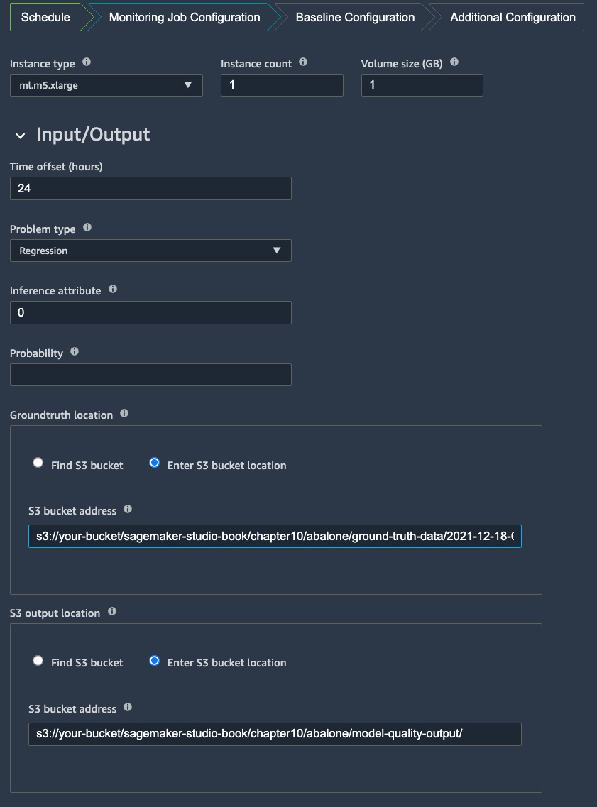
Figure 10.7 – Setting up input and output for the model quality monitor

Input refers to both model prediction from the endpoint and the ground-truth files we are uploading in the notebook. In the Input/Output options, Time offset (hours) refers to hours allowed to wait for ground-truth labels to become available in S3. We know that typically, there is a delay between the prediction event occurring and the outcome of the event becoming available. This offset addresses that delay and allows Model Monitor to look out for the corresponding ground truth for a prediction event. Because we are generating the inference data and the ground-truth label at the same time from the notebook, we can safely use the default value—24 hours. For Problem type, we choose Regression from the drop-down list as the model predicts the ring size and age of an abalone. In Inference attribute and Probability, we inform SageMaker how to interpret the model prediction from the endpoint. Depending on the output format, CSV or JSON, we would put in either the index location or JSON path, respectively. Because our model returns a regression value in CSV format and does not return a probability score, we would put 0 for Inference attribute to specify the first value being the model output, and leave Probability empty.

Note

If the content type for your model is JSON/JSON Lines, you would specify a JSON path in Inference attribute and Probability. For example, when a model returns {prediction: {"predicted_label":1, "probability":0.68}}, you would specify "prediction.predicted_label" in Inference attribute while specifying "prediction.probability" in Probability.

For Groundtruth location, we use the S3 location where we uploaded the ground-truth labels. It's in the ground_truth_upload_path variable in the notebook. For S3 output location, we specify an S3 bucket location for Model Monitor to save the output. Lastly, you can optionally configure the encryption and VPC for the monitoring jobs. Click Continue to proceed.

10. On the third page, Baseline Configuration, as shown in Figure 10.8, we specify the baseline data for the baselining. We have created baseline data from the validation set. Let's provide the S3 location of the CSV file that is saved in the model_quality_baseline_s3 variable in the notebook to the Baseline dataset S3 location field. For Baseline S3 output location, we provide an S3 location to save the baselining result. Choose CSV with header in Baseline dataset format. Leave the instance type and configuration as the default.

This is to configure the SageMaker Processing job for the one-time baseline computation. In the last three fields, we put the corresponding CSV header names—Rings for Baseline groundtruth attribute and Prediction for Baseline inference attribute—and leave the field empty for Baseline probability because, again, our model does not produce probability. Click Continue:

Figure 10.8 – Configuring the baseline calculation for the model quality monitor

11. In Additional Configuration, we can provide preprocessing and postprocessing scripts to the monitor like in the case of the data quality monitor. Let's skip this and proceed to complete the setup by clicking Enable model monitoring.

Now, we have created the model quality monitor. You can see the monitoring schedule is in the Scheduled status under the Model quality tab on the ENDPOINT DETAILSpage. Similar to the data quality monitor, a baseline processing job is launched to compute the baseline model performance using the baseline dataset. An hourly monitoring job will also be launched as a SageMaker Processing job within 20 minutes at the top of an hour in order to compute the model performance metrics from the inference data gathered during the hour and compare them against the baseline. We will review the monitoring results in the next section, Reviewing model monitoring results in SageMaker Studio.

Reviewing model monitoring results in SageMaker Studio

SageMaker Model Monitor computes various statistics on the incoming inference data, compares them against the precomputed baseline statistics, and reports the results back to us in a specified S3 bucket, which you can visualize in SageMaker Studio.

For the data quality monitor, a SageMaker Model Monitor pre-built, default container, which is what we used, computes per-feature statistics on the baseline dataset and the inference data. The statistics include the mean, sum, standard deviation, min, and max. The data quality monitor also looks at data missingness and checks for the data type of the incoming inference data. You can find the full list at https://docs.aws.amazon.com/sagemaker/latest/dg/model-monitor-interpreting-statistics.html.

For the model quality monitor, SageMaker computes model performance metrics based on the ML problem type configured. For our regression example in this chapter, SageMaker's model quality monitor is computing the mean absolute error (MAE), mean squared error (MSE), root mean square error (RMSE), and R-squared (r2) values. You can find the full list of computed metrics for regression, binary classification, and multi-class classification problems at https://docs.aws.amazon.com/sagemaker/latest/dg/model-monitor-model-quality-metrics.html.

You can see a list of the monitoring jobs launched over time in the Monitoring job history tab on the ENDPOINT DETAILS page, as shown in Figure 10.9:

Figure 10.9 – Viewing a list of monitoring jobs. Double-clicking a row item takes you to the detail page of a particular job

When you double-click a row item, you will be taken to the detail page of a particular monitoring job, as shown in Figure 10.10. Because we perturbed the data prior to sending it to the endpoint, the data contains irregularities, such as missingness. This is captured by the data quality monitor:

Figure 10.10 – Details of a data quality monitoring job and violations

We can also open a model quality monitoring job to find out whether the model performs as expected. As shown in Figure 10.11, we can see that violations have been raised for all the metrics computed. We know it is going to happen because this is largely due to the perturbation we introduced to the data. SageMaker Model Monitor is able to detect such problems:

Figure 10.11 – Details of a model monitoring job and violations

We can also create visualizations from the monitoring jobs. Let's follow the next steps to create a chart for the data quality monitor:

1. On the ENDPOINT DETAILS page, go to the Data quality tab and click on the Add chart button, as shown in Figure 10.12:

Figure 10.12 – Adding a visualization for a data quality monitor

2. A chart properties configuration sidebar will appear on the right side, as shown in Figure 10.13. We can create a chart by specifying the timeline, the statistics, and the feature we would like to plot. Depending on how long you've enabled the monitor, you can choose a time span to visualize. For example, I chose 1 day, the Average statistic, and feature_baseline_drift_Length to see the average baseline drift measure on the Length feature in the past day:

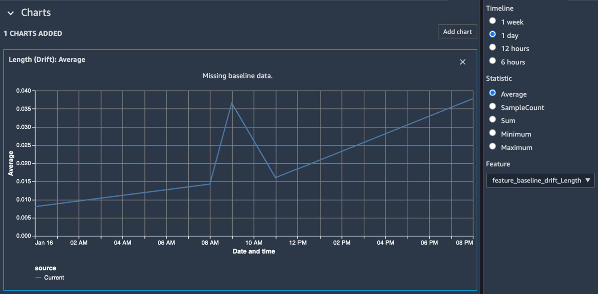
Figure 10.13 – Visualizing feature drift in SageMaker Studio

3. You can optionally add more charts by clicking the Add chart button.
4. Similarly, we can visualize the model performance using the mse metric over the last 24 hours, as shown in Figure 10.14:

Figure 10.14 – Visualizing the mse regression metric in SageMaker Studio

Note

To save costs, when you complete the examples, make sure to uncomment and run the last cells in 01-train_host_predict.ipynb to delete the monitoring schedules and the endpoint in order to stop incurring charges to your AWS account.

Summary

In this chapter, we focused on data drift and model drift in ML and how to monitor them using SageMaker Model Monitor and SageMaker Studio. We demonstrated how we set up a data quality monitor and a model quality monitor in SageMaker Studio to continuously monitor the behavior of a model and the characteristics of the incoming data, in a scenario where a regression model is deployed in a SageMaker endpoint and continuous inference traffic is hitting the endpoint. We introduced some random perturbation to the inference traffic and used SageMaker Model Monitor to detect unwanted behavior of the model and data. With this example, you can also deploy SageMaker Model Monitor to your use case and provide visibility and a guardrail to your models in production.

In the next chapter, we will be learning how to operationalize an ML project with SageMaker Projects, Pipelines, and the model registry. We will be talking about an important trend in ML right now, that is, continuous integration/continuous delivery (CI/CD) and ML operations (MLOps). We will demonstrate how you can use SageMaker features, such as Projects, Pipelines, and the model registry, to make your ML project repeatable, reliable, and reusable, and have strong governance.