
Chapter 7: Hosting ML Models in the Cloud: Best Practices
After you've successfully trained a model, you want to make the model available for inference, don't you? ML models are often the product of a business that is ML-driven. Your customers consume the ML prediction from your model, not your training jobs or processed data. How do you provide a satisfying customer experience, starting with a good experience with your ML models?
SageMaker has several options for ML hosting and inferencing, depending on your use case. Options are welcomed in many aspects of life, but it can be difficult to find the best option. This chapter will help you understand how to host models for batch inference and for online real-time inference, how to use multi-model endpoints to save costs, and how to conduct resource optimization for your inference needs.
In this chapter, we will be covering the following topics:
- Deploying models in the cloud after training
- Inferencing in batches with batch transform
- Hosting real-time endpoints
- Optimizing your model deployment
Technical requirements
For this chapter, you need to access the code at https://github.com/PacktPublishing/Getting-Started-with-Amazon-SageMaker-Studio/tree/main/chapter07. If you did not run the notebooks in the previous chapter, please run the chapter05/02-tensorflow_sentiment_analysis.ipynb file from the repository before proceeding.
Deploying models in the cloud after training
ML models can primarily be consumed in the cloud in two ways, batch inference and live inference. Batch inference refers to model inference performed on data that is in batches, often large batches, and asynchronous in nature. It fits use cases that collect data infrequently, that focus on group statistics rather than individual inference, and that do not need to have inference results right away for downstream processes. Projects that are research oriented, for example, do not require model inference to be returned for a data point right away. Researchers often collect a chunk of data for testing and evaluation purposes and care about overall statistics and performance rather than individual predictions. They can conduct the inference in batches and wait for the prediction for the whole batch to complete before they move on.
Live inference, on the other hand, refers to model inference performed in real time. It is expected that the inference result for an incoming data point is returned immediately so that it can be used for subsequent decision-making processes. For example, an interactive chatbot would require a live inference capability to support such a service. No one would want to wait until the end of the conversation to get responses from the chatbot model, nor would people want to wait for more than even a couple of seconds. Companies looking to provide the best customer experience would want an inference to be made and returned to the customer instantly.
Given the different requirements, the architecture and deployment choices also differ between batch inference and live inference. Amazon SageMaker has it covered as it provides various fully managed options for your inference use cases. SageMaker batch transform is designed to perform batch inference at scale and is cost-effective as the compute infrastructure is fully managed and is de-provisioned when your inference job is complete. SageMaker real-time endpoints aim to provide a robust live hosting option for your ML use cases. Both the SageMaker hosting options are fully managed, meaning you do not have to worry much about the cloud infrastructure.
Let's first take a look at SageMaker batch transform, how it works, and when to use it.
Inferencing in batches with batch transform
SageMaker batch transform is designed to provide offline inference for large datasets. Depending on how you organize the data, SageMaker batch transform can split a single large text file in S3 by lines into a small and manageable size (mini-batch) that would fit into the memory before making inference against the model; it can also distribute the files by S3 key into compute instances for efficient computation. For example, it could send test1.csv to instance 1 and test2.csv to instance 2.
To demonstrate SageMaker batch transform, we can pick up from our training example in the previous chapter. In Chapter 6, Detecting ML Bias and Explaining Models with SageMaker Clarify, we showed you how to train a TensorFlow model using SageMaker managed training for a movie review sentiment prediction use case in Getting-Started-with-Amazon-SageMaker-Studio/chapter05/02-tensorflow_sentiment_analysis.ipynb. We can deploy the trained model to make a batch inference using SageMaker batch transform in the following steps:
- Please open the Getting-Started-with-Amazon-SageMaker-Studio/chapter07/01-tensorflow_sentiment_analysis_batch_transform.ipynb notebook and use the Python 3 (TensorFlow 2.3 Python 3.7 CPU Optimized) kernel.
- Run the first three cells to set up the SageMaker SDK, import the libraries, and prepare the test dataset. There are 25,000 documents in the test dataset. We save the test data as a CSV file and upload the CSV file to our S3 bucket. The file is 27 MB.
Note
SageMaker batch transform expects the input CSV files to not contain headers. That is, the first row of the CSV should be the first data point.
- We retrieve the training TensorFlow estimator from a training job we did in Chapter 6, Detecting ML Bias and Explaining Models with SageMaker Clarify. We need to grab the training job name for the TensorFlow.attach() method. You can find it in Experiments and trials in the left sidebar, as shown in Figure 7.1, thanks to the experiments we used when training. In Experiments and trials, left-click on imdb-sentiment-analysis and you should see your training job as a trial in the list.

Figure 7.1 – Obtaining training job name in Experiments and trials
You should replace training_job_name in the following code with your own:
from sagemaker.tensorflow import TensorFlow
training_job_name='<your-training-job-name>'
estimator = TensorFlow.attach(training_job_name)
Once you have replaced training_job_name and attached it to reload estimator, you should see the history of the job printed in the output.
- To run SageMaker batch transform, you only need two lines of SageMaker API code:
transformer = estimator.transformer(instance_count=1,
instance_type='ml.c5.xlarge',
max_payload = 2, # MB
accept = 'application/jsonlines',
output_path = s3_output_location,
assemble_with = 'Line')
transformer.transform(test_data_s3,
content_type='text/csv',
split_type = 'Line',
job_name = jobname,
experiment_config = experiment_config)
The estimator.transformer() method creates a Transformer object with the compute resource desired for the inference. Here we request one ml.c5.xlarge instance for predicting 25,000 movie reviews. The max_payload argument allows us to control the size of each mini-batch that SageMaker Batch Transform is splitting. The accept argument determines the output type. SageMaker managed Tensorflow serving container supports 'application/json', and 'application/jsonlines'. assemble_with controls how you assemble the inference results that are in mini-batches. Then we provide the S3 location of the test data (test_data_s3) in the transformer.transform(), and indicate that the input content type to be of 'text/csv' as the file is of CSV format. split_type determines how the input files will be split by SageMaker Batch Transform into mini-batch. We put in a unique job name and SageMaker Experiments configuration so that we can track the inference to the associated training job in the same trial. The Batch Transform job would take around 5 minutes to complete. Like a training job, SageMaker manages the provisioning, computation, and de-provisioning of the instances once the job finishes.
- After the job completes, we should take a look at the result. SageMaker batch transform saves the results after assembly to the specified S3 location with .out appended to the input filename. You can access the full S3 path in transformer.output_path attribute. SageMaker uses TensorFlow Serving, a model serving framework developed by TensorFlow, for model serving, the model output is written in JSON format. The output has the sentiment probabilities in an array with predictions as the JSON key. We can inspect the batch transform results with the following code:
output = transformer.output_path
output_prefix = 'imdb_data/test_output'
!mkdir -p {output_prefix}
!aws s3 cp --recursive {output} {output_prefix}
!head {output_prefix}/{csv_test_filename}.out
{ "predictions": [[0.00371244829], [1.0], [1.0], [0.400452465], [1.0], [1.0], [0.163813606], [0.10115058], [0.793149233], [1.0], [1.0], [6.37737814e-14], [2.10463966e-08], [0.400452465], [1.0], [0.0], [1.0], [0.400452465], [2.65155926e-29], [4.04420768e-11], ……]}
We then collect all 25,000 predictions into a results variable:
results=[]
with open(f'{output_prefix}/{csv_test_filename}.out', 'r') as f:
lines = f.readlines()
for line in lines:
print(line)
json_output = json.loads(line)
result = [float('%.3f'%(item)) for sublist in json_output['predictions']
for item in sublist]
results += result
print(results)
- The rest of the notebook displays one original movie review, the predicted sentiment, and the corresponding ground truth sentiment. The model returns the probabilities of the reviews being positive or negative. We take a 0.5 threshold and mark probabilities over the threshold to be positive and below 0.5 to be negative.
- As we logged the batch transform job in the same trial as the training job, we can find it easily in Experiments and trials in the left sidebar, as shown in Figure 7.2. You can see more information about this batch transform job in this entry.
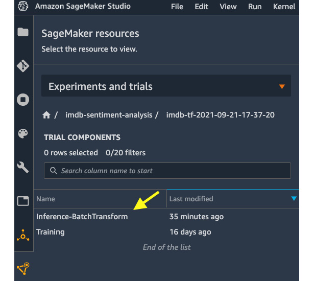
Figure 7.2 – The batch transform job is logged as a trial component alongside the training component
That's how easy it is to make use of SageMaker batch transform to generate inferences on a large dataset. You may wonder, why can't I just use the notebook to make inferences? What's the benefit of using SageMaker batch transform? Yes, you can use the notebook for quick analysis. The advantages of SageMaker batch transform are as follows:
- Fully managed mini-batching helps make inferences on a large dataset efficiently.
- You can use a separate SageMaker-managed compute infrastructure that is different from your notebook instance. You can easily run prediction with a cluster of instances for faster prediction.
- You only pay for the runtime of a batch transform job, even with a much larger compute cluster.
- You can schedule and kick off a model prediction independently in the cloud with SageMaker batch transform. It is not necessary to use a Python notebook in SageMaker Studio to start a prediction job.
Next, let's see how we can host ML models in the cloud for real-time use cases.
Hosting real-time endpoints
SageMaker real-time inference is a fully managed feature for hosting your model(s) on compute instance(s) for real-time low-latency inference. The deployment process consists of the following steps:
- Create a model, container, and associated inference code in SageMaker. The model refers to the training artifact, model.tar.gz. The container is the runtime environment for the code and the model.
- Create an HTTPS endpoint configuration. This configuration carries information about compute instance type and quantity, models, and traffic patterns to model variants.
- Create ML instances and an HTTPS endpoint. SageMaker creates a fleet of ML instances and an HTTPS endpoint that handles the traffic and authentication. The final step is to put everything together for a working HTTPS endpoint that can interact with client-side requests.
Hosting a real-time endpoint faces one particular challenge that is common when hosting a website or a web application: it can be difficult to scale your compute instances when you have a spike in traffic to your endpoint. You may have 1,000 customers visiting your website per minute in a particular hour and then have 100,000 customers in the next hour. If you only deploy one instance behind your endpoint that is capable of handling 5,000 requests per minute, it would work well in the first hour and would struggle in the next. Autoscaling is a technique in the cloud to help you scale out instances automatically when certain criteria are met so that your application can handle the load at any time.
Let's walk through a SageMaker real-time endpoint example. Like the batch transform example, we continue the ML use case in Chapter 5, Building and Training ML Models with SageMaker Studio IDE and 05/02-tensorflow_sentiment_analysis. ipynb. Please open the notebook in Getting-Started-with-Amazon-SageMaker-Studio/chapter07/02-tensorflow_sentiment_analysis_inference.ipynb and use the Python 3 (TensorFlow 2.3 Python 3.7 CPU Optimized) kernel. We will deploy a trained model to SageMaker as a real-time endpoint, make some predictions as an example, and finally apply an autoscaling policy to help scale the compute instances behind the endpoint. Please follow these steps:
- In the first four cells, we set up the SageMaker session, load the Python libraries, load the test data that we created in 01-tensorflow_sentiment_analysis_batch_transform.ipynb, and retrieve the training job that we trained previously using its name.
- We then deploy the model to an endpoint:
predictor = estimator.deploy(
instance_type='ml.c5.xlarge',
initial_instance_count=1)
Here, we choose ml.c5.xlarge for instance_type argument. initial_instance_ count argument refers to the number of ML instances behind the endpoint when we make this call. Later, we will show you how to use the autoscaling feature, which is designed to help us scale out the instance fleet when the initial settings become insufficient. The deployment process takes about 5 minutes.
- We can test the endpoint with some sample data. The TensorFlow Serving framework in the container handles the data interface and takes the NumPy array as input so we can pass an entry into the model directly. We can get a response from the endpoint in JSON format, which gets converted to a dictionary in Python in the prediction variable:
prediction=predictor.predict(x_test[data_index])
print(prediction)
{'predictions': [[1.80986511e-11]]}
The next two cells retrieve the review in text and print out the ground truth sentiment and the predicted sentiment with a threshold of 0.5, just like in the batch transform example.
- (Optional) You may be wondering: Can I ask the endpoint to predict the entire x_test of 25,000 data points? To find out, feel free to try out the following line:
predictor.predict(x_test)
This line will run for a couple of seconds and eventually fail. This is because a SageMaker endpoint is designed to take on requests that are 6 MB in size one at a time. You can request inferences for multiple data points, for example, x_test[:100], but not 25,000 all in one call. In contrast, batch transform does the data splitting (mini-batching) automatically and is better suited to handle large datasets.
- Next, we can apply SageMaker's autoscaling feature to this endpoint using the application-autoscaling client from the boto3 SDK:
sagemaker_client = sess.boto_session.client('sagemaker')
autoscaling_client = sess.boto_session.client('application-autoscaling')
- It is a two-step process to configure autoscaling for computing instances in AWS. First, we run autoscaling_client.register_scalable_target() to register the target with the desired minimum/maximum capacity for our SageMaker endpoint:
resource_id=f'endpoint/{endpoint_name}/variant/AllTraffic'
response = autoscaling_client.register_scalable_target(
ServiceNamespace='sagemaker',
ResourceId=resource_id,
ScalableDimension='sagemaker:variant:DesiredInstanceCount',
MinCapacity=1,
MaxCapacity=4)
Our target, the SageMaker real-time endpoint, is denoted with resource_id. We set the minimum capacity to 1 and the maximum to 4, meaning that when the load is at the lowest, there will be at least one instance running behind the endpoint. Our endpoint is capable of scaling out to four instances at the most.
- Then we run autoscaling_client.put_scaling_policy() to instruct how we want to autoscale:
response = autoscaling_client.put_scaling_policy(
PolicyName='Invocations-ScalingPolicy',
ServiceNamespace='sagemaker',
ResourceId=resource_id,
ScalableDimension='sagemaker:variant:DesiredInstanceCount',
PolicyType='TargetTrackingScaling',
TargetTrackingScalingPolicyConfiguration={
'TargetValue': 4000.0,
'PredefinedMetricSpecification': {
'PredefinedMetricType':
'SageMakerVariantInvocationsPerInstance'},
'ScaleInCooldown': 600,
'ScaleOutCooldown': 300})
In this example, we employ a scaling strategy called target tracking scaling. Target tracking scaling aims to scale in and out the instances based on a specific target metric, such as instance CPU load, or the number of inference requests per instance per minute. We use the latter (SageMakerVariantInvocationsPerInstance) in this configuration to make sure each instance can share 4,000 requests per minute before scaling out another instance. ScaleInCooldown and ScaleOutCooldown refer to the period of time in seconds after the last scaling activity before autoscaling can scale in and out again. With our configuration, SageMaker will not scale in (remove an instance) within 600 seconds of the last scale-in activity, and will not scale out (add an instance) within 300 seconds of the last scale-out activity.
Note
There are two commonly used advanced scaling strategies for PolicyType: step scaling and scheduled scaling. In step scaling, you can define the number of instances to scale in/out based on the size of the alarm breaches of a certain metric. Read more about step scaling at https://docs.aws.amazon.com/autoscaling/ec2/userguide/as-scaling-simple-step.html. In scheduled scaling, you can set up the scaling based on the schedule. This is particularly useful if the traffic is predictable or has some seasonality. Read more about scheduled scaling at https://docs.aws.amazon.com/autoscaling/ec2/userguide/schedule_time.html.
- We can verify the configuration of the autoscaling policy with the following code:
response = autoscaling_client.describe_scaling_policies(
ServiceNamespace='sagemaker')
for i in response['ScalingPolicies']:
print('')
print(i['PolicyName'])
print('')
if('TargetTrackingScalingPolicyConfiguration' in i):
print(i['TargetTrackingS calingPolicyConfiguration'])
else:
print(i['StepScalingPolicyConfiguration'])
print('')
Invocations-ScalingPolicy
{'TargetValue': 4000.0, 'PredefinedMetricSpecification': {'PredefinedMetricType': 'SageMakerVariantInvocationsPerInstance'}, 'ScaleOutCooldown': 300, 'ScaleInCooldown': 600}
- In Amazon SageMaker Studio, you can easily find the details of an endpoint in the Endpoints registry in the left sidebar, as shown in Figure 7.3. If you double-click on an endpoint, you can see more information in the main working area:
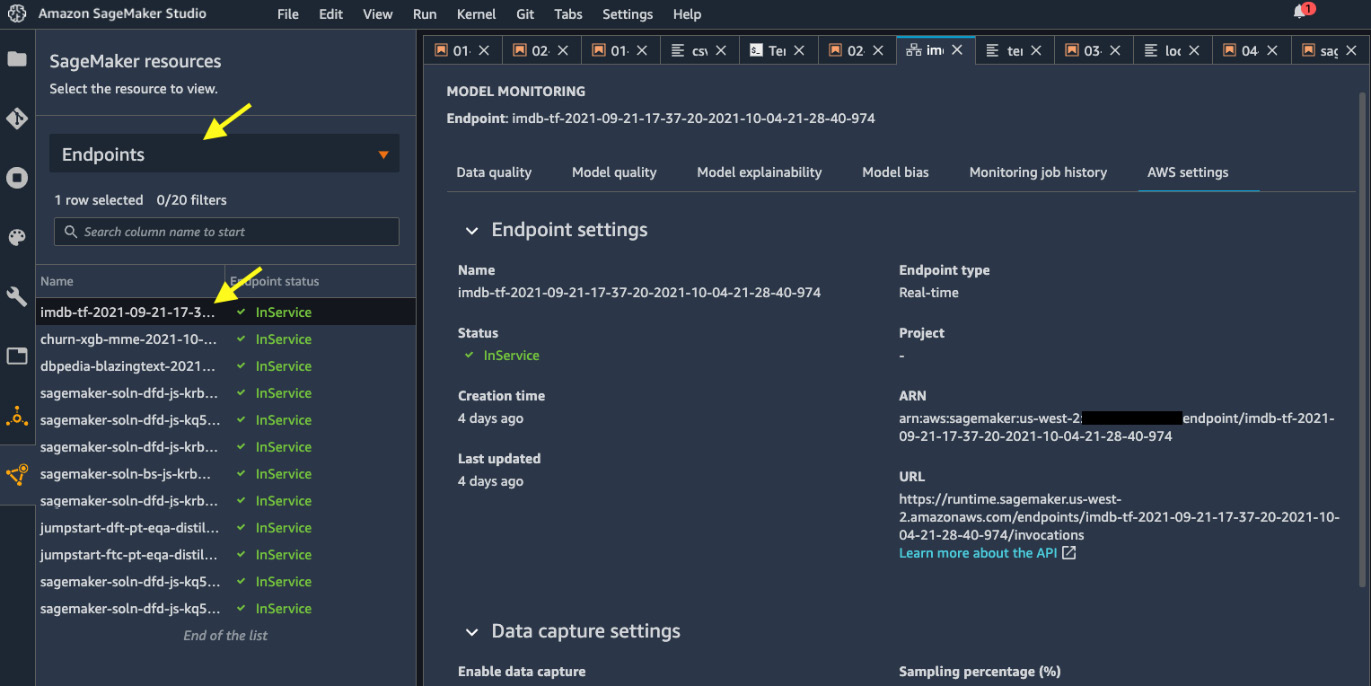
Figure 7.3 – Discovering endpoints in SageMaker Studio
The purpose of hosting an endpoint is to serve the ML models in the cloud so that you can integrate ML as a microservice into your applications or websites. Your model has to be available at all times as long as your main product or service is available. You can imagine that there is a great opportunity and incentive for you to optimize the deployment to minimize the cost while maintaining performance. We just learned how to deploy an ML model in the cloud; we should also learn how to optimize the deployment.
Optimizing your model deployment
Optimizing model deployment is a critical topic for businesses. No one wants to be spending a dime more than they need to. Because deployed endpoints are being used continuously, and incurring charges continuously, making sure that the deployment is optimized in terms of cost and runtime performance can save you a lot of money. SageMaker has several options to help you reduce costs while optimizing the runtime performance. In this section, we will be discussing multi-model endpoint deployment and how to choose the instance type and autoscaling policy for your use case.
Hosting multi-model endpoints to save costs
A multi-model endpoint is a type of real-time endpoint in SageMaker that allows multiple models to be deployed behind the same endpoint. There are many use cases in which you would build models for each customer or for each geographic area, and depending on the characteristics of the incoming data point, you would apply the corresponding ML model. Take the telecommunications churn prediction use case that we tackled in Chapter 3, Data Preparation with SageMaker Data Wrangler, as an example. We may get more accurate ML models if we train them by state because there may be regional differences in terms of competition among local telecommunication providers. And if we do train ML models for each US state, you can also easily imagine that the utilization of each model might not be completely equal. Actually, quite the contrary.
Model utilization is inevitably proportional to the population of each state. Your New York model is going to be used more frequently than your Alaska model. In this scenario, if you host an endpoint for each state, you will have to pay for instances, even for the least utilized endpoint. With multi-model endpoints, SageMaker helps you reduce costs by reducing the number of endpoints needed for your use case. Let's take a look at how it works with the telecommunications churn prediction use case. Please open the Getting-Started-with-Amazon-SageMaker-Studio/chapter07/03-multimodel-endpoint.ipynb notebook with the Python 3 (Data Science) kernel and follow the next steps:
- We define the SageMaker session, load up the Python libraries, and load the churn dataset in the first three cells.
- We do minimal preprocessing to convert the binary columns from strings to 0 and 1:
df[["Int'l Plan", "VMail Plan"]] = df[["Int'l Plan", "VMail Plan"]].replace(to_replace=['yes', 'no'], value=[1, 0])
df['Churn?'] = df['Churn?'].replace(to_replace=['True.', 'False.'], value=[1, 0])
- We leave out 10% of the data for ML inference later on:
from sklearn.model_selection import train_test_split
df_train, df_test = train_test_split(df_processed,
test_size=0.1, random_state=42, shuffle=True,
stratify=df_processed['State'])
- After the data is prepared, we set up our state-wise model training process in the function launch_training_job() with SageMaker Experiments integrated. The training algorithm we use is SageMaker's built-in XGBoost algorithm, which is fast and accurate for structural data like this. For binary classification, we use a binary:logtistic objective with num_round set to 20:
def launch_training_job(state, train_data_s3, val_data_s3):
...
xgb = sagemaker.estimator.Estimator(image, role,
instance_count=train_instance_count,
instance_type=train_instance_type,
output_path=s3_output,
enable_sagemaker_metrics=True,
sagemaker_session=sess)
xgb.set_hyperparameters(
objective='binary:logistic',
num_round=20)
...
xgb.fit(inputs=data_channels,
job_name=jobname,
experiment_config=experiment_config,
wait=False)
return xgb
- With launch_training_job(), we could easily create multiple training jobs in a for loop for states. For demonstration purposes, we only train five states in this example:
dict_estimator = {}
for state in df_processed.State.unique()[:5]:
print(state)
output_dir = f's3://{bucket}/{prefix}/{local_prefix}/by_state'
df_state = df_train[df_train['State']==state].drop(labels='State', axis=1)
df_state_train, df_state_val = train_test_split(df_state, test_size=0.1, random_state=42,
shuffle=True, stratify=df_state['Churn?'])
df_state_train.to_csv(f'{local_prefix}/churn_{state}_train.csv', index=False)
df_state_val.to_csv(f'{local_prefix}/churn_{state}_val.csv', index=False)
sagemaker.s3.S3Uploader.upload(f'{local_prefix}/churn_{state}_train.csv', output_dir)
sagemaker.s3.S3Uploader.upload(f'{local_prefix}/churn_{state}_val.csv', output_dir)
dict_estimator[state] = launch_training_job(state, out_train_csv_s3, out_val_csv_s3)
time.sleep(2)
Each training job should take no more than 5 minutes. We will wait for all of them to complete before proceeding to use the wait_for_training_job_to_complete() function.
- After the training is done, we finally deploy our multi-model endpoint. It's a bit different to deploying a single model to an endpoint from a trained estimator object. We use the sagemaker.multidatamodel.MultiDataModel class for deployment:
model_PA = dict_estimator['PA'].create_model(
role=role, image_uri=image)
mme = MultiDataModel(name=model_name,
model_data_prefix=model_data_prefix,
model=model_PA,
sagemaker_session=sess)
MultiDataModel initialization needs to understand the common model configuration, such as the container image and the network configurations, to configure the endpoint configuration. We pass in the model for PA. Afterward, we deploy the model to one ml.c5.xlarge instance and configure the serializer and deserializer to take CSV as input and produce JSON as output, respectively:
predictor = mme.deploy(
initial_instance_count=hosting_instance_count,
instance_type=hosting_instance_type,
endpoint_name=endpoint_name,
serializer = CSVSerializer(),
deserializer = JSONDeserializer())
- We can then dynamically add models to the endpoint. Note that at this time, there is no model deployed behind an endpoint:
for state, est in dict_estimator.items():
artifact_path = est.latest_training_job.describe()['ModelArtifacts']['S3ModelArtifacts']
model_name = f'{state}.tar.gz'
mme.add_model(model_data_source=artifact_path,
model_data_path=model_name)
That's it. We can verify that there are five models associated with this endpoint:
list(mme.list_models())
['MO.tar.gz', 'PA.tar.gz', 'SC.tar.gz', 'VA.tar.gz', 'WY.tar.gz']
- We can test out the endpoint with some data points from each state. You can specify which model to make inference with using the target_model argument in predictor.predict():
state='PA'
test_data=sample_test_data(state)
prediction = predictor.predict(data=test_data[0],
target_model=f'{state}.tar.gz')
In this cell and onwards, we also set up a timer to measure the time it takes models for other states to respond in order to illustrate the nature of dynamic loading of the model from S3 to the endpoint. When the endpoint is first created, there is no model located behind the endpoint. With add_model(), it merely upload the models to an S3 location, model_data_prefix. When a model is first requested, SageMaker dynamically downloads the requested model from S3 to the ML instance and loads it into the inference container. This process has a longer response time when we first run the prediction for each of the state models, up to 1,000 milliseconds. But once the model is loaded into the memory in the container behind the endpoint, the response time is greatly reduced, to around 20 milliseconds. When a model is loaded, it is persisted in the container until the memory of the instance is exhausted by having too many models loaded at once. Then SageMaker unloads models that are not being used anymore from memory while still keeping model.tar.gz on disk in the instance for the next request to avoid downloading it from S3.
In this example, we showed how to host a SageMaker multi-model endpoint that is flexible and cost-effective because it drastically reduces the number of endpoints needed for your use case. So, instead of hosting and paying for five endpoints, we would only host and pay for one endpoint. That's an easy 80% cost saving. With hosting models trained for 50 US states in 1 endpoint instead of 50, that's a 98% cost saving!
With SageMaker multi-model endpoints, you can host as many models as you can in an S3 bucket location. The number of simultaneous models you can load in an endpoint depends on the memory footprint of your models and the amount of RAM on the compute instance. Multi-model endpoints are suitable for use cases where you have models that are built in the same framework (XGBoost in this example), and where it is tolerable to have latency on less frequently used models.
Note
If you have models built from different ML frameworks, for example, a mix of TensorFlow, PyTorch, and XGBoost models, you can use a multi-container endpoint, which allows hosting up to 15 distinct framework containers. Another benefit of multi-container endpoints is that they do not have latency penalties as all containers are running at the same time. Find out more at https://docs.aws.amazon.com/sagemaker/latest/dg/multi-container-endpoints.html.
The other optimization approach is using a technique called load testing to help us choose the instance and autoscaling policy.
Optimizing instance type and autoscaling with load testing
Load testing is a technique that allows us to understand how our ML model hosted in an endpoint with a compute resource configuration responds to online traffic. There are factors such as model size, ML framework, number of CPUs, amount of RAM, autoscaling policy, and traffic size that affect how your ML model performs in the cloud. Understandably, it's not easy to predict how many requests can come to an endpoint over time. It is prudent to understand how your model and endpoint behave in this complex situation. Load testing creates artificial traffic and requests to your endpoint and stress tests how your model and endpoint respond in terms of model latency, instance CPU utilization, memory footprint, and so on.
In this section, let's run some load testing against the endpoint we created in chapter07/02-tensorflow_sentiment_analysis_inference.ipynb with some scenarios. In the example, we hosted a TensorFlow-based model to an ml.c5.xlarge instance, which has 4 vCPUs and 8 GiB of memory.
First of all, we need to understand the model's latency and capacity as a function of the type of instance and the number of instances before an endpoint becomes unavailable. Then we vary the instance configuration and autoscaling configuration until the desired latency and traffic capacity has been reached.
Please open the Getting-Started-with-Amazon-SageMaker-Studio/chapter07/04-load_testing.ipynb notebook with the Python 3 (Data Science) kernel and an ml.t3.xlarge instance and follow these steps:
- We use a Python load testing framework called locust to perform the load testing in SageMaker Studio. Let's download the library first in the notebook. You can read more about the library at https://docs.locust.io/en/stable/index.html.
- As usual, we set up the SageMaker session in the second cell.
- Create a load testing configuration script, load_testing/locustfile.py, which is required by locust. The script is also provided within the repository. This cell overwrites the file. In this configuration, we instruct locust to create simulated users (the SMLoadTestUser class) to run model inference against a SageMaker endpoint (the test_endpoint class function) provided by the environment variable with a data point loaded from imdb_data/test/test.csv. Here, the response time, total_time, is measured in milliseconds (ms).
- In the next cell, we start our first load testing job on our already-deployed SageMaker endpoint with an ml.c5.xlarge instance. Remember we applied the autoscaling policy in chapter07/02-tensorflow_sentiment_analysis_inference? Let's first reverse the policy by setting MaxCapacity to 1 to make sure the endpoint does not scale out to multiple instances during our first test:
sagemaker_client = sess.boto_session.client('sagemaker')
autoscaling_client = sess.boto_session.client('application-autoscaling')
endpoint_name = '<endpoint-with-ml.c5-xlarge-instance>'
resource_id = f'endpoint/{endpoint_name}/variant/AllTraffic'
response = autoscaling_client.register_scalable_target(
ServiceNamespace='sagemaker',
ResourceId=resource_id,
ScalableDimension='sagemaker:variant: DesiredInstanceCount',
MinCapacity=1,
MaxCapacity=1)
- Then we test the endpoint with locust. We set up two-worker distributed load testing on two CPU cores in the following snippet. We instruct locust to create 10 users (the -r 10 argument) per second up to 500 online users (-u 500), each making calls to our endpoint for 60 seconds (-t 60s). Please replace the ENDPOINT_NAME string with your SageMaker endpoint name. You can find the endpoint name in the Endpoints registry, as shown in Figure 7.3:
%%sh --bg
export ENDPOINT_NAME='<endpoint-with-ml.c5-xlarge-instance>'
bind_port=5557
locust -f load_testing/locustfile.py --worker --loglevel ERROR --autostart --autoquit 10 --master-port ${bind_port} &
locust -f load_testing/locustfile.py --worker --loglevel ERROR --autostart --autoquit 10 --master-port ${bind_port} &
locust -f load_testing/locustfile.py --headless -u 500 -r 10 -t 60s
--print-stats --only-summary --loglevel ERROR
--autostart --autoquit 10 --master --expect-workers 2 --master-bind-port ${bind_port}
As it is running, let's navigate to the Amazon CloudWatch console to see what's happening from the endpoint's perspective. Please copy the following URL and replace <endpoint-with-ml.c5-xlarge-instance> with your endpoint name and replace the region if you use a region other than us-west-2: https://us-west-2.console.aws.amazon.com/cloudwatch/home?region=us-west-2#metricsV2:graph=~(metrics~(~(~'AWS*2fSageMaker~'InvocationsPerInstance~'EndpointName~'<endpoint-with-ml.c5-xlarge-instance>~'VariantName~'AllTraffic)~(~'.~'ModelLatency~'.~'.~'.~'.~(stat~'Average))~(~'.~'Invocations~'.~'.~'.~'.)~(~'.~'OverheadLatency~'.~'.~'.~'.~(stat~'Average))~(~'.~'Invoca tion5XXErrors~'.~'.~'.~'.)~(~'.~'Invocation4XXErrors~'.~'.~'.~'.))~view~'timeSeries~stacked~false~region~'us-west-2~stat~'Sum~period~60~start~'-PT3H~end~'P0D );query=~'*7bAWS*2fSageMaker*2cEndpointName*2cVariantName*7d*20<endpoint-with-ml.c5-xlarge-instance>
You can see a dashboard in Figure 7.4. The dashboard has captured the most important metrics regarding our SageMaker endpoint's health and status. Invocations and InvocationsPerInstance show the total number of invocations and per-instance counts. Invocation5XXErrors and Invocation4XXErrors are error counts with HTTP codes 5XX and 4XX respectively. ModelLatency (in microseconds) is the time taken by a model inside the container behind a SageMaker endpoint to return a response. OverheadLatency (in microseconds) is the time taken for our SageMaker endpoint to transmit a request and a response. Total latency for a request is ModelLatency plus OverheadLatency. These metrics are emitted by our SageMaker endpoint to Amazon CloudWatch.
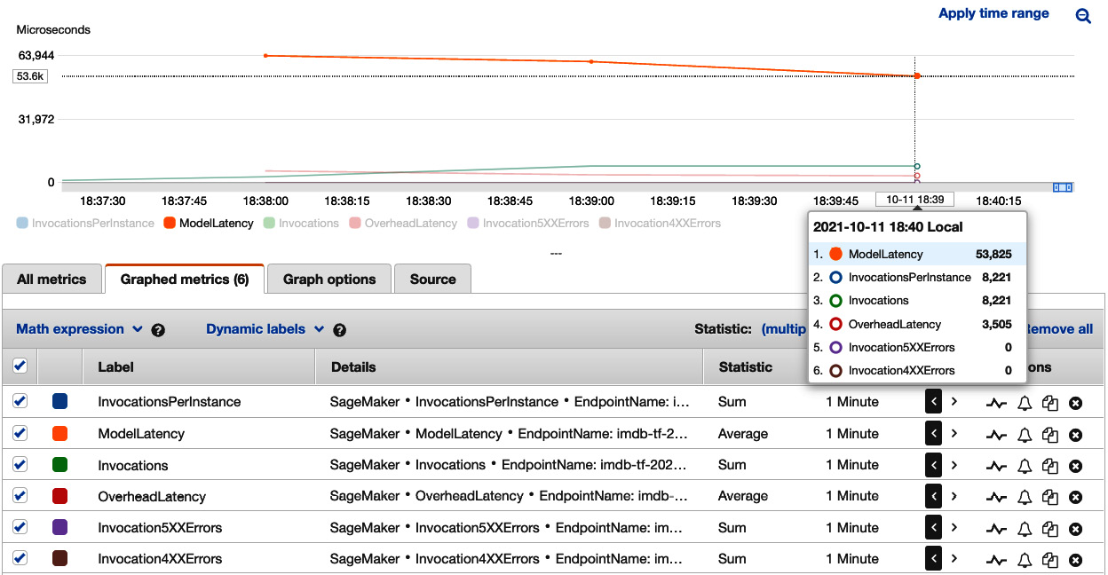
Figure 7.4 – Viewing load testing results on one ml.c5.xlarge instance in Amazon CloudWatch
In the first load test (Figure 7.4), we can see that there are around 8,221 invocations per minute, 0 errors, with an average ModelLatency of 53,825 microseconds, or 53.8 milliseconds.
With these numbers in mind as a baseline, let's scale up the instance, that is, let's use a larger instance.
- We load up the previous IMDb sentiment analysis training job and deploy the TensorFlow model to another endpoint with one ml.c5.2xlarge instance, which has 8 vCPU and 16 GiB of memory, twice the capacity of ml.c5.xlarge:
from sagemaker.tensorflow import TensorFlow
training_job_name='<your-training-job-name>'
estimator = TensorFlow.attach(training_job_name)
predictor_c5_2xl = estimator.deploy(
initial_instance_count=1,
instance_type='ml.c5.2xlarge')
The deployment process takes a couple of minutes. Then we retrieve the endpoint name with the next cell, predictor_c5_2xl.endpoint_name.
- Replace ENDPOINT_NAME with the output of predictor_c5_2xl.endpoint_name and run the cell to kick off another load test against the new endpoint:
export ENDPOINT_NAME='<endpoint-with-ml.c5-2xlarge-instance>'
- In Amazon CloudWatch (replacing <endpoint-with-ml.c5-xlarge- instance> in the long URL in step 4 or clicking the hyperlink generated in the next cell in the notebook), we can see how the endpoint responds to traffic in Figure 7.5:
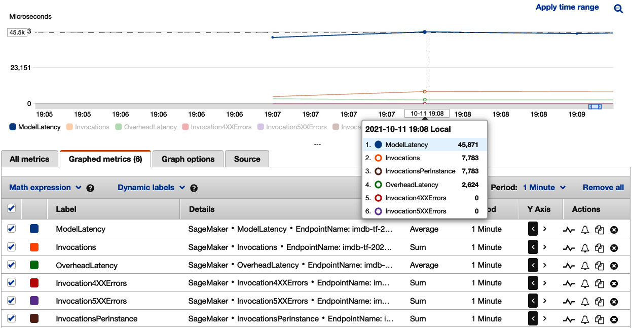
Figure 7.5 – Viewing load testing results on one ml.c5.2xlarge instance in Amazon CloudWatch
Similarly, the traffic that locust was able to generate is around 8,000 invocations per minute (7,783 in Figure 7.5). ModelLatency clocks at 45,871 microseconds (45.8 milliseconds), which is 15% faster than the result from one ml.c5.xlarge instance.
- Next, we deploy the same model to an ml.g4dn.xlarge instance, which is a GPU instance dedicated to model inference use cases. G4dn instances are equipped with NVIDIA T4 GPUs and are cost-effective for ML inference and small neural network training jobs:
predictor_g4dn_xl = estimator.deploy(
initial_instance_count=1,
instance_type='ml.g4dn.xlarge')
- We set up a load testing job similar to the previous ones. The result can also be found on the Amazon CloudWatch dashboard by replacing <endpoint-with-ml.c5-xlarge- instance> in the long URL in step 4 or clicking the hyperlink generated in the next cell in the notebook. As shown in Figure 7.6, with around 6,000 invocations per minute, the average ModelLatency is 2,070 microseconds (2.07 milliseconds). This is significantly lower than the previous compute configurations, thanks to the GPU device in the ml.g4dn.xlarge instance making inference much faster.
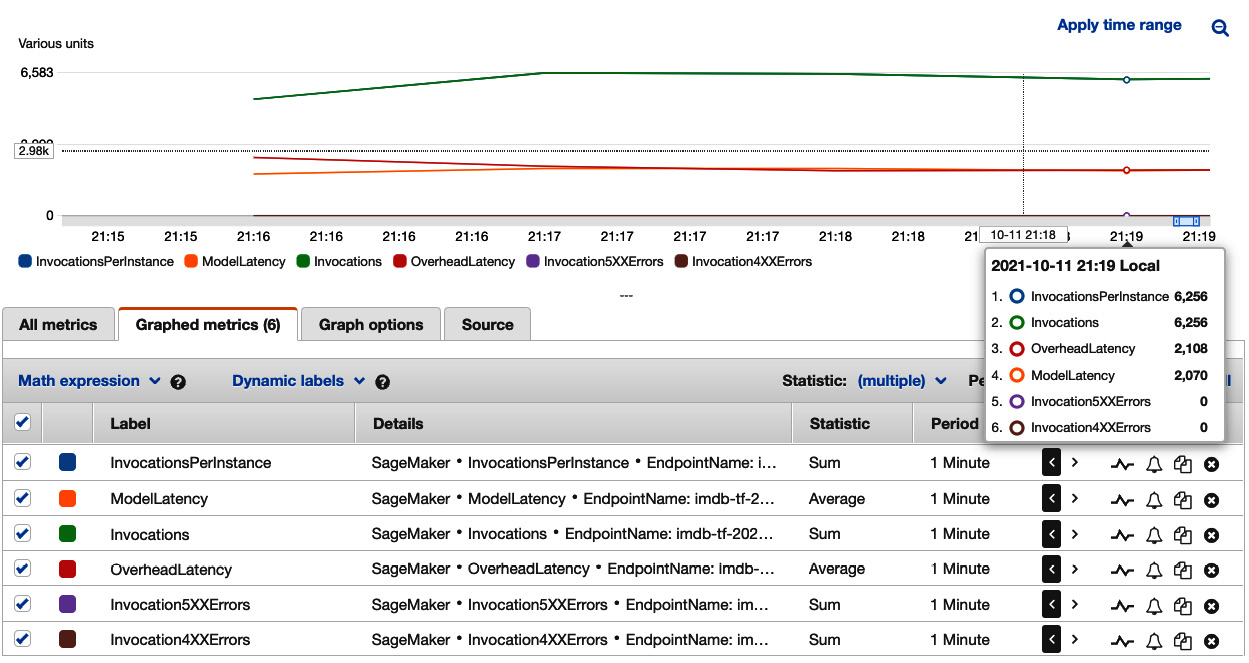
Figure 7.6 – Viewing the load test results on one ml.g4dn.xlarge instance in Amazon CloudWatch
- The last approach we should try is autoscaling. Autoscaling allows us to spread the load across instances, which in turns helps improve the CPU utilization and model latency. We once again set the autoscaling to MaxCapacity=4 with the following cell:
endpoint_name = '<endpoint-with-ml.c5-xlarge-instance>'
resource_id=f'endpoint/{endpoint_name}/variant/AllTraffic'
response = autoscaling_client.register_scalable_target(
ServiceNamespace='sagemaker',
ResourceId=resource_id,
ScalableDimension='sagemaker:variant:DesiredInstanceCount',
MinCapacity=1,
MaxCapacity=4)
You can confirm the scaling policy attached with the next cell in the notebook.
- We are ready to perform our last load testing experiment. Replace ENDPOINT_NAME with <endpoint-with-ml.c5-xlarge-instance>, and run the next cell to kick off the load test against the endpoint that is now able to scale out up to four instances. This load test needs to run longer in order to see the effect of autoscaling. This is because SageMaker first needs to observe the number of invocations to decide how many new instances are based on our target metric, SageMakerVariantInvocationsPerInstance=4000. With our traffic at around 8,000 invocations per minute, SageMaker will spin up one additional instance to have a per-instance invocation at the desired value, 4,000. Spinning up new instances takes around 5 minutes to complete.
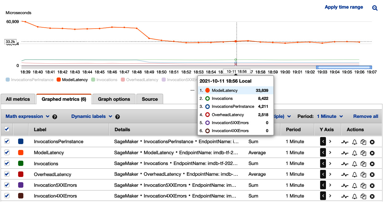
Figure 7.7 – Viewing load testing results on an ml.c5.xlarge instance with autoscaling in Amazon CloudWatch
We can see the load test result on the Amazon CloudWatch dashboard, as shown in Figure 7.7. We can see an interesting pattern in the chart. We can clearly see something happened between 18:48 and 18:49. The ModelLatency dropped significantly from around 50,000 microseconds (50 milliseconds) to around 33,839 microseconds (33.8 milliseconds). And the InvocationsPerInstance was cut to half the number of Invocations. We are seeing the effect of SageMaker's autoscaling. Instead of one single instance taking all 8,000 invocations, SageMaker determines that two instances are more appropriate to achieve a target of SageMakerVariantInvocationsPerInstance=4000 and splits the traffic into two instances. A lower ModelLatency is the preferred outcome of having multiple instances to share the load.
After the four load testing experiments, we can conclude that at a load of around 6,000 to 8,000 invocations per minute, the following takes place:
- Single-instance performance is measured by average ModelLatency. ml.g4dn.xlarge with 1 GPU and 4 vCPUs gives the smallest ModelLatency at 2.07 milliseconds. Next is the ml.c5.2xlarge instance with 8 vCPUs at 45.8 milliseconds. Last is the ml.c5.xlarge instance with 4 vCPUs at 53.8 milliseconds.
- With autoscaling, two ml.c5.xlarge instances with 8 vCPUs achieves 33.8 milliseconds' ModelLatency. This latency is even better than having one ml.c5.2xlarge with the same number of vCPUs.
If we consider another dimension, the cost of the instance(s), we can come to an even more interesting situation, as shown in Figure 7.8. In the table, we create a simple compound metric to measure the cost-performance efficiency of a configuration by multiplying ModelLatency by the price per hour of the instance configuration.
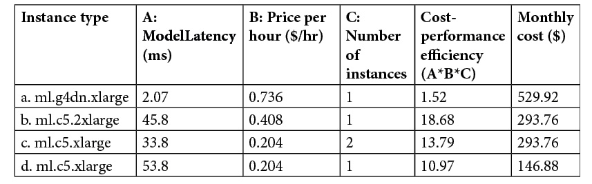
Figure 7.8 – Cost-performance comparisons
If we are constrained by cost, we should consider using the last configuration (row d), where the monthly cost is the lowest yet with the second-best cost-performance efficiency while sacrificing some model latency. If we need a model latency of around 40 milliseconds or lower, by paying the same monthly cost, we would get even more bang for our buck and lower latency with the third configuration (row c) than the second configuration (row b). The first configuration (row a) gives the best model latency and the best cost-performance efficiency. But it is also the most expensive option. Unless there is a strict single-digit model latency requirement, we might not want to use this option.
To reduce cost, when you complete the examples, make sure to uncomment and run the last cells in 02-tensorflow_sentiment_analysis_inference.ipynb, 03-multimodel-endpoint.ipynb, and 04-load_testing.ipynb to delete the endpoints in order to stop incurring charges to your AWS account.
This discussion is based on the example we used, which assumes many factors, such as model framework, traffic pattern, and instance types. You should follow the best practices we introduced for your use case and test out more instance types and autoscaling policies to find the optimal solution for your use case. You can find the full list of instances, specifications, and prices per hour in the real-time inference tab at https://aws.amazon.com/sagemaker/pricing/ to come up with your own cost-performance efficiency analysis.
There are other optimization features in SageMaker that help you reduce latency, such as Amazon Elastic Inference, SageMaker Neo, and Amazon EC2 Inf1 instances. Elastic Inference (https://docs.aws.amazon.com/sagemaker/latest/dg/ei-endpoints.html) attaches fractional GPUs to a SageMaker hosted endpoint. It increases the inference throughput and decreases the model latency for your deep learning models that can benefit from GPU acceleration. SageMaker Neo (https://docs.aws.amazon.com/sagemaker/latest/dg/neo.html) optimizes an ML model for inference in the cloud and supported devices at the edge with no loss in accuracy. SageMaker Neo speeds up prediction and reduces cost with a compiled model and optimized container in SageMaker hosted endpoint. Amazon EC2 Inf1 instances (https://aws.amazon.com/ec2/instance-types/inf1/) provide high performance and low cost in the cloud with AWS Inferentia chips designed and built by AWS for ML inference purposes. You can compile supported ML models using SageMaker Neo and select Inf1 instances to deploy the compiled model in a SageMaker hosted endpoint.
Summary
In this chapter, we learned how to efficiently make ML inferences in the cloud using Amazon SageMaker. We followed up with what we trained in the previous chapter—an IMDb movie review sentiment prediction—to demonstrate SageMaker's batch transform and real-time hosting. More importantly, we learned how to optimize for cost and model latency with load testing. We also learned about another great cost-saving opportunity by hosting multiple ML models in one single endpoint using SageMaker multi-model endpoints. Once you have selected the best inference option and instance types for your use case, SageMaker makes deploying your models straightforward. With these step-by-step instructions and this discussion, you will be able to translate what you've learned to your own ML use cases.
In the next chapter, we will take a different route to learn how we can use SageMaker's JumpStart and Autopilot to quick-start your ML journey. SageMaker JumpStart offers solutions to help you see how best practices and ML use cases are tackled. JumpStart model zoos collect numerous pre-trained deep learning models for natural language processing and computer vision use cases. SageMaker Autopilot is an autoML feature that crunches data and trains a performant model without you worrying about data, coding, or modeling. After we have learned the fundamentals of SageMaker—fully managed model training and model hosting—we can better understand how SageMaker JumpStart and Autopilot work.