
Chapter 5: Building and Training ML Models with SageMaker Studio IDE
Building and training a machine learning (ML) model can be easy with SageMaker Studio. It is an integrated development environment (IDE) designed for ML developers for building and training ML models at scale and efficiently. In order to train an ML model, you may previously have dealt with the cumbersome overhead of managing compute infrastructure for yourself or for your team to train ML models properly. You may also have experienced compute resource constraints, either on desktop machines or with cloud resources, where you are given a fixed-size instance. When you develop in SageMaker Studio, there is no more frustration with provisioning and managing compute infrastructure because you can easily make use of elastic compute in SageMaker Studio and its wide support of sophisticated ML algorithms and frameworks for your ML use case.
In this chapter, we will be covering the following topics:
- Training models with SageMaker's built-in algorithms
- Training with code written in popular frameworks
- Developing and collaborating using SageMaker Notebook
Technical requirements
For this chapter, you need to access the code provided at https://github.com/PacktPublishing/Getting-Started-with-Amazon-SageMaker-Studio/tree/main/chapter05.
Training models with SageMaker's built-in algorithms
When you want to build an ML model from a notebook in SageMaker Studio for your ML use case and data, one of the easiest approaches is to use one of SageMaker's built-in algorithms. There are two advantages of using built-in algorithms:
- The built-in algorithms do not require you to write any sophisticated ML code. You only need to provide your data, make sure the data format matches the algorithms' requirements, and specify the hyperparameters and compute resources.
- The built-in algorithms are optimized for AWS compute infrastructure and are scalable out of the box. It is easy to perform distributed training across multiple compute instances and/or enable GPU support to speed up training time.
SageMaker's built-in algorithm suite offers algorithms that are suitable for the most common ML use cases. There are algorithms for the following categories: supervised learning, unsupervised learning, image analysis, and textual analysis. Most notably, there is XGBoost and k-means for tabular data for supervised learning and unsupervised learning, respectively, as well as image classification, object detection, and semantic segmentation for image analysis. For textual analysis, we have the word2vec, text classification, and sequence-to-sequence algorithms. These are just example algorithms for each category we've mentioned. There are more useful algorithms available but I am not listing them exhaustively. You can visit https://docs.aws.amazon.com/sagemaker/latest/dg/algos.html to see a full list and further details.
Note
GPU support and distributed training capability for algorithms vary. Please visit https://docs.aws.amazon.com/sagemaker/latest/dg/common-info-all-im-models.html for GPU and distributed training support for each algorithm.
Let's take a use case and an algorithm to demonstrate how to use SageMaker's built-in algorithms.
Training an NLP model easily
Training an ML model does not require writing any ML codes with SageMaker's built-in algorithms. We will look at an NLP use case to classify sentences into categories using the DBpedia Ontology Dataset from DBpedia (https://www.dbpedia.org/), which consists of 560,000 training samples and 70,000 testing samples of the titles and abstracts of Wikipedia articles. Please open the notebook in chapter05/01-built_in_algorithm_text_classification.ipynb from the repository using the Python 3 (Data Science) kernel and the ml.t3.medium instance.
In the notebook, we first download the dataset and inspect it to understand how we need to process the data, as shown in the following snippet:
!wget -q https://github.com/le-scientifique/torchDatasets/raw/master/dbpedia_csv.tar.gz
!tar -xzf dbpedia_csv.tar.gz
!head dbpedia_csv/train.csv -n 3
!cat dbpedia_csv/classes.txt
We see that the data, dbpedia_csv/train.csv, is formatted as <class index>,<title>,<abstract>. There is also a file called dbpedia_csv/classes.txt documenting the classes in an order that corresponds to the class index seen in dbpedia_csv/train.csv.
This is a text classification problem: given the abstract of an article, we want to build a model to predict and classify the classes this abstract belong to. This is a common use case when working with a large number of text documents, such as articles on the Wikipedia site from which this dataset is sourced. It is almost impossible to use human review to organize all the documents.
One of the built-in algorithms that is suitable for this use case is BlazingText. BlazingText has highly optimized implementations for both Word2vec (unsupervised) and text classification (supervised). The Word2vec algorithm can convert text into a vector representation, or word embedding, for any downstream NLP usage, such as sentiment analysis or named entity recognition. Text classification can classify documents into categories. This is perfect for our use case and dataset.
Getting the data ready for training is key when using SageMaker's built-in algorithm. Using BlazingText for text classification requires each data point to be formatted as __label__<class> text…. Here's an example:
__label__latin Lorem ipsum dolor sit amet , consectetur adipiscing elit , sed do eiusmod tempor incididunt ut labore et dolore magna aliqua .
We use a preprocess function, which calls the transform_text function to tokenize each row of the abstract. We use a sentence tokenizer, punkt, from the nltk library inside the transform_text function. We preprocess both train and test files. To keep the processing time manageable, we use only 20% of the training data, as shown in the following code snippet:
preprocess("dbpedia_csv/train.csv", "dbpedia.train", keep=0.2)
preprocess("dbpedia_csv/test.csv", "dbpedia.validation")
!head -n 1 dbpedia.train
__label__Company automatic electric automatic electric company ( ae ) was the largest of the manufacturing units of the automatic electric group . it was a telephone equipment supplier for independent telephone companies in north america and also had a world-wide presence . with its line of automatic telephone exchanges it was also a long-term supplier of switching equipment to the bell system starting in 1919.
We can see that now we have the data in the expected format. Feel free to expand the training set to a higher percentage using the keep argument in preprocess. After preprocessing, we are ready to invoke the built-in algorithm.
SageMaker's built-in algorithms are fully managed containers that can be accessed with a simple SDK call. The following code allows us to use the BlazingText algorithm for text classification:
image=sagemaker.image_uris.retrieve(framework='blazingtext',
region=region,
version='1')
print(image)
433757028032.dkr.ecr.us-west-2.amazonaws.com/blazingtext:1
After execution, we get a string in a variable called image. You may be wondering, what is this string that looks like a URL path? How is this an algorithm for model training?
Container technology is the core of SageMaker managed training. Container technology allows SageMaker the flexibility to work with algorithms from any framework and any runtime requirements. Instead of using the runtime setup in the notebook and using the compute resource behind the notebook for model training, SageMaker takes the data you supply and a container image that has the runtime setup and the code base to a separate SageMaker-managed compute infrastructure to conduct model training.
The path in image points to a container image stored in Amazon Elastic Container Registry (ECR) that has the BlazingText ML algorithm. We can use it to start a model training job with a SageMaker estimator.
SageMaker estimator is a key construct for the fully managed model training that enables us to command various aspects of a model training job with a simple API. The following snippet is how we set up a training job with SageMaker's BlazingText algorithm:
estimator = sagemaker.estimator.estimator(
image,
role,
instance_count=1,
instance_type='ml.c5.2xlarge',
volume_size=30,
max_run=360000,
input_mode='File',
enable_sagemaker_metrics=True,
output_path=s3_output_location,
hyperparameters={
'mode': 'supervised',
'epochs': 20,
'min_count': 2,
'learning_rate': 0.05,
'vector_dim': 10,
'early_stopping': True,
'patience': 4,
'min_epochs': 5,
'word_ngrams': 2,
},
)
Most notably, the arguments that go into the estimator are as follows:
- The algorithm as a container, image
- hyperparameters for the training job
- The compute resources needed for the job, instance_type, instance_count, and volume_size
- The IAM execution role, role
As you can see, not only do we specify algorithmic options, but also instruct SageMaker what cloud compute resources we need for this model training run. We request one ml.c5.2xlarge instance, a compute-optimized instance that has high-performance processors, with 30 GB storage for this training job. It allows us to use a lightweight, cheap instance type (ml.t3.medium) for the notebook environment during prototyping and do full-scale training on a more powerful instance type to get the job done faster.
We have set up the algorithm and the compute resource; next, we need to associate the estimator with the training data. After we have prepared the data, we need to upload the data into an S3 bucket so that the SageMaker training job can access the ml.c5.4xlarge instance. We start the training by simply calling estimator.fit() with the data:
train_channel = prefix + '/train'
validation_channel = prefix + '/validation'
sess.upload_data(path='dbpedia_csv/dbpedia.train', bucket=bucket, key_prefix=train_channel)
sess.upload_data(path='dbpedia_csv/dbpedia.validation', bucket=bucket, key_prefix=validation_channel)
s3_train_data = f's3://{bucket}/{train_channel}'
s3_validation_data = f's3://{bucket}/{validation_channel}'
print(s3_train_data)
print(s3_validation_data)
data_channels = {'train': s3_train_data,
'validation': s3_validation_data}
exp_datetime = strftime('%Y-%m-%d-%H-%M-%S', gmtime())
jobname = f'dbpedia-blazingtext-{exp_datetime}'
estimator.fit(inputs=data_channels,
job_name=jobname,
logs=True)
You can see the job log in the notebook and observe the following:
- SageMaker spins up one ml.c5.2xlarge instance for this training job.
- SageMaker downloads the data from S3 and the BlazingText container image from ECR.
- SageMaker runs the model training and logs the training and validation accuracy in the cell output shown here:
#train_accuracy: 0.9961
Number of train examples: 112000
#validation_accuracy: 0.9766
Number of validation examples: 70000
The cell output from the training job is also available in Amazon CloudWatch Logs. The metrics of the training job, such as CPU utilization and accuracy measures, which we enabled in estimator(…, enable_sagemaker_metrics=True), are sent to Amazon CloudWatch Metrics automatically. This gives us governance of the training jobs even if the notebooks are accidentally deleted.
Once the training job finishes, you can access the trained model in estimator.model_data, which can later be used for hosting and inferencing either in the cloud, which is a topic we will explore in depth in the next chapter, or on a computer with the fastText program. You can access the model with the following code block:
!aws s3 cp {estimator.model_data} ./dbpedia_csv/
%%sh
cd dbpedia_csv/
tar -zxf model.tar.gz
# Use the model archive with fastText
# eg. fasttext predict ./model.bin test.txt
Note
BlazingText is a GPU-accelerated version of FastText. FastText (https://fasttext.cc/) is an open source library that can perform both word embedding generation (unsupervised) and text classification (supervised). The models created by BlazingText and FastText are compatible with each other.
We have just created a sophisticated text classification model that is capable of classifying the category of documents from DBpedia at an accuracy of 0.9766 on the validation data with minimal ML code.
Let's also set up an ML experiment management framework, SageMaker Experiments, to keep track of jobs we launch in this chapter.
Managing training jobs with SageMaker Experiments
As data scientists, we might have all encountered a tricky situation where the number of model training runs can grow very quickly to such a degree that it becomes difficult to track the best model in various experiment settings, such as dataset versions, hyperparameters, and algorithms. In SageMaker Studio, you can easily track the experiments among the training runs with SageMaker Experiments and visualize them in the experiments and trials component UI. SageMaker Experiments is an open source project (https://github.com/aws/sagemaker-experiments) and can be accessed programmatically through the Python SDK.
In SageMaker Experiments, an Experiment is a collection of trial runs that are executions of an ML workflow that can contain trial components such as data processing and model training.
Let's continue with the chapter05/01-built_in_algorithm_text_classification.ipynb notebook and see how we can set up an experiment and trial with SageMaker Experiments to track training jobs with different learning rates in the following snippet so that we can compare the performance from the trials easily in SageMaker Studio:
- First, we install the sagemaker-experiments SDK in the notebook kernel:
!pip install -q sagemaker-experiments
- We then create an experiment named dbpedia-text-classification that we can use to store all the jobs related to this model training use case using the smexperiments library:
from smexperiments.experiment import Experiment
from smexperiments.trial import Trial
from botocore.exceptions import ClientError
from time import gmtime, strftime
import time
experiment_name = 'dbpedia-text-classification'
try:
experiment = Experiment.create(
experiment_name=experiment_name,
description='Training a text classification model using dbpedia dataset.')
except ClientError as e:
print(f'{experiment_name} experiment already exists! Reusing the existing experiment.')
- Then we create a utility function, create_estimator(), with an input argument, learning_rate, for ease of use later when we iterate over various learning rates:
def create_estimator(learning_rate):
hyperparameters={'mode': 'supervised',
'epochs': 40,
'min_count': 2,
'learning_rate': learning_rate,
'vector_dim': 10,
'early_stopping': True,
'patience': 4,
'min_epochs': 5,
'word_ngrams': 2}
estimator = sagemaker.estimator.estimator(
image,
role,
instance_count=1,
instance_type='ml.c4.4xlarge',
volume_size=30,
max_run=360000,
input_mode='File',
enable_sagemaker_metrics=True,
output_path=s3_output_location,
hyperparameters=hyperparameters)
return estimator
- Let's run three training jobs in a for loop with varying learning rates in order to understand how the accuracy changes:
for lr in [0.1, 0.01, 0.001]:
exp_datetime = strftime('%Y-%m-%d-%H-%M-%S', gmtime())
jobname = f'dbpedia-blazingtext-{exp_datetime}'
exp_trial = Trial.create(
experiment_name=experiment_name,
trial_name=jobname)
experiment_config={
'ExperimentName': experiment_name,
'TrialName': exp_trial.trial_name,
'TrialComponentDisplayName': 'Training'}
estimator = create_estimator(learning_rate=lr)
estimator.fit(inputs=data_channels,
job_name=jobname,
experiment_config=experiment_config,
wait=False)
In the for loop, we create unique training job names, dbpedia-blazingtext-{exp_datetime}, to be associated with a trial, exp_trial, and an experiment configuration, experiment_config, to store information. Then we pass experiment_config into the estimator.fit() function and SageMaker will track the experiments for us automatically.
Note
We put wait=False in the estimator.fit() call. This allows the training job to run asynchronously, meaning that the cell is returned immediately as opposed to being held by the process until the training is completed. In effect, our jobs with different learning rates are run in parallel, each using its own separate SageMaker-managed instances for training.
In SageMaker Studio, you can easily compare the results of these training jobs with SageMaker Experiments. We can create a chart to compare the accuracies of the three jobs with varying learning rates in the SageMaker Studio UI:
- Click on the SageMaker Components and registries in the left sidebar, as shown in Figure 5.1:
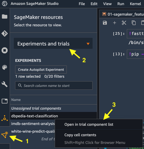
Figure 5.1 – Viewing experiments and trials from the left sidebar
- Select Experiments and trials in the drop-down menu, as shown in Figure 5.1.
- Right-click on the dbpedia-text-classification experiment entry and choose Open in trial component list.
- A new view in the main working area will pop up. You can configure the columns to show the accuracies and learning rates as shown in Figure 5.2. We can see validation:accuracy, and train:accuracy with respect to the three learning_rate settings. With learning_rate set to 0.01, we have the most balanced training and validation accuracies. A learning rate of 0.1 is overfitted, while a learning rate of 0.001 is underfitted.
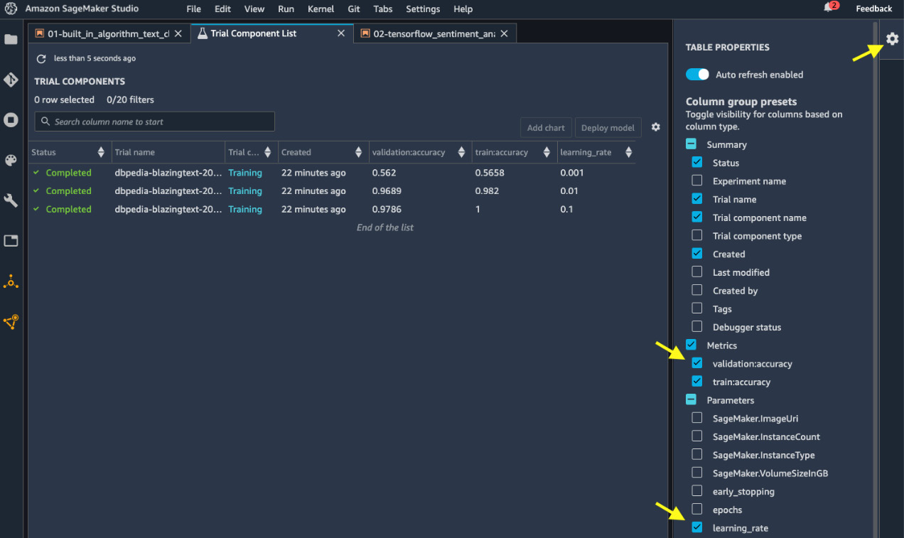
Figure 5.2 – Viewing and comparing training jobs
- We can create a line chart of validation:accuracy versus learning_rate. Multi-select the three trial components and click Add chart in the top right. A new view will pop up. Configure the chart properties as shown in Figure 5.3. You will get a chart that shows the relationship between validation:accuracy and learning_rate.
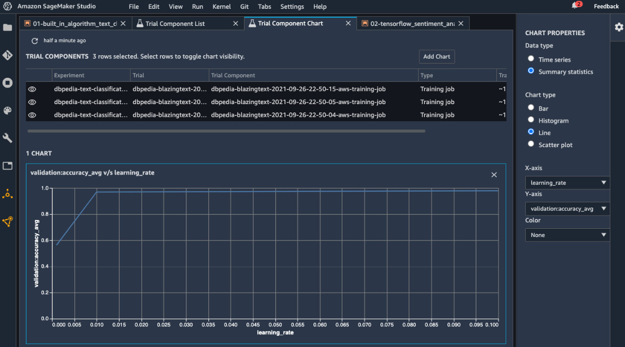
Figure 5.3 – Comparing and charting validation accuracy versus learning rate
SageMaker Experiments is useful for managing jobs and resources and comparing performance as you start building an ML project at scale in SageMaker Studio.
Note
Training and processing jobs that do not have experiment_config will be placed in Unassigned trial components.
More often than not, you already have some ML projects that use popular frameworks such as TensorFlow and PyTorch to train models. You can also run them with SageMaker's fully managed training capability.
Training with code written in popular frameworks
SageMaker's fully managed training works with your favorite ML frameworks too, thanks to the container technology we mentioned previously. You may have been working with Tensorflow, PyTorch, Hugging Face, MXNet, scikit-learn, and many more. You can easily use them with SageMaker so that you can use its fully managed training capabilities and benefit from the ease of provisioning right-sized compute infrastructure. SageMaker enables you to use your own training scripts for custom models and run them on prebuilt containers for popular frameworks. This is known as Script Mode. For frameworks not covered by the prebuilt containers, you also can use your own container for virtually any framework of your choice.
Let's look at training a sentiment analysis model written in TensorFlow as an example to show you how to use your own script in SageMaker to run with SageMaker's prebuilt TensorFlow container. Then we will describe a similar process for other frameworks.
TensorFlow
TensorFlow is an open source framework for ML, specifically for deep neural networks. You can run TensorFlow code using SageMaker's prebuilt TensorFlow training and inference containers, available through the SageMaker SDK's sagemaker.tensorflow. Please open the notebook in chapter05/02-tensorflow_sentiment_analysis.ipynb from the repository using the Python 3 (TensorFlow 2.3 Python 3.7 CPU Optimized) kernel and the ml.t3.medium instance. The objective in this example is to train and predict the sentiment (positive/negative) from movie reviews from the IMDb movie database using a neural network built with TensorFlow layers. You could run the neural network training inside a notebook, but this will require you to have a compute instance that is capable of training a deep neural network with a large amount of data at all times, even when you are just exploring data and writing code. But with SageMaker, you can optimize the compute usage by using a smaller instance for code building and only using a GPU instance for full-scale training.
In chapter06/02-tensorflow_sentiment_analysis.ipynb, we first install the library we need and get the Sagemaker session set up. Then we load the IMDb dataset from tensorflow.python.keras.datasets, run minimal data preprocessing, and save the training and test splits to the local filesystem and then to an S3 bucket.
Assuming we have previously developed a neural network architecture that works on this IMDb dataset, as shown in the following code block, we can easily take it into SageMaker to train.
embedding_layer = tf.keras.layers.Embedding(max_features,
embedding_dims,
input_length=maxlen)
sequence_input = tf.keras.Input(shape=(maxlen,), dtype='int32')
embedded_sequences = embedding_layer(sequence_input)
x = tf.keras.layers.Dropout(args.drop_out_rate)(embedded_sequences)
x = tf.keras.layers.Conv1D(filters, kernel_size, padding='valid', activation='relu', strides=1)(x)
x = tf.keras.layers.MaxPooling1D()(x)
x = tf.keras.layers.GlobalMaxPooling1D()(x)
x = tf.keras.layers.Dense(hidden_dims, activation='relu')(x)
x = tf.keras.layers.Dropout(drop_out_rate)(x)
preds = tf.keras.layers.Dense(1, activation='sigmoid')(x)
model = tf.keras.Model(sequence_input, preds)
optimizer = tf.keras.optimizers.Adam(learning_rate)
model.compile(loss='binary_crossentropy', optimizer=optimizer, metrics=['accuracy'])
SageMaker can take a TensorFlow script into a Docker container and train the script with the data. To do so, SageMaker requires the script to be aware of environmental variables set in the container, the compute infrastructure, and, optionally, the script needs to be able to take inputs from the execution, such as hyperparameters. Here are the steps:
- Create a script to put in the model architecture and data loading functions (get_model, get_train_data, get_test_data, and so on).
- Create an argument parser that takes in parameters such as hyperparameters and training data location from script execution. SageMaker is going to run the script as an executable in the container with arguments specified from a SDK call. The training data location is passed into the script with a default from environmental variable SageMaker set up in the container (SM_CHANNEL_*). The argument parser is defined in a parse_arg() function, shown as follows:
def parse_args():
parser = argparse.ArgumentParser()
# hyperparameters sent by the client are passed as command-line arguments to the script
parser.add_argument('--epochs', type=int, default=1)
parser.add_argument('--batch_size', type=int, default=64)
parser.add_argument('--learning_rate', type=float, default=0.01)
parser.add_argument('--drop_out_rate', type=float, default=0.2)
# data directories
parser.add_argument('--train', type=str, default=os.environ.get('SM_CHANNEL_TRAIN'))
parser.add_argument('--test', type=str, default=os.environ.get('SM_CHANNEL_TEST'))
# model directory /opt/ml/model default set by SageMaker
parser.add_argument('--model_dir', type=str, default=os.environ.get('SM_MODEL_DIR'))
return parser.parse_known_args()
Note
The TRAIN or TEST suffix in the SM_CHANNEL_* environmental variable has to match that of the dictionary key provided in the input data channel in the estimator.fit() call. So, later, when we specify the data channel, we need to create a dictionary whose keys are TRAIN and TEST, case-insensitive.
- Put in the training steps as part of if __name__ == "__main__"::
if __name__ == "__main__":
args, _ = parse_args()
x_train, y_train = get_train_data(args.train)
x_test, y_test = get_test_data(args.test)
model = get_model(args)
history = model.fit(x_train, y_train,
batch_size=args.batch_size,
epochs=args.epochs,
validation_data=(x_test, y_test))
save_history(args.model_dir + "/history.p", history)
# create a TensorFlow SavedModel for deployment to a SageMaker endpoint with TensorFlow Serving
model.save(args.model_dir + '/1')
- Make sure to replace the variables in the network with that from the argument parser. For example, change tf.keras.optimizers.Adam(learning_rate) to tf.keras.optimizers.Adam(args.learning_rate).
- In our notebook, we write out the script to code/tensorflow_sentiment.py.
- Create a TensorFlow estimator using sagemaker.tensorflow.TensorFlow, which is an extension of the estimator class we used previously to work exclusively with ML training written in TensorFlow:
from sagemaker.tensorflow import TensorFlow
exp_datetime = strftime('%Y-%m-%d-%H-%M-%S', gmtime())
jobname = f'imdb-tf-{exp_datetime}'
model_dir = f's3://{bucket}/{prefix}/{jobname}'
code_dir = f's3://{bucket}/{prefix}/{jobname}'
train_instance_type = 'ml.p3.2xlarge'
hyperparameters = {'epochs': 10, 'batch_size': 256, 'learning_rate': 0.01 , 'drop_out_rate': 0.2 }
estimator = TensorFlow(source_dir='code',
entry_point='tensorflow_sentiment.py',
model_dir=model_dir,
code_location=code_dir,
instance_type=train_instance_type,
instance_count=1,
enable_sagemaker_metrics=True,
hyperparameters=hyperparameters,
role=role,
framework_version='2.1',
py_version='py3')
Some of the key arguments here in TensorFlow estimator are source_dir, entry_point, code_location, framework_version, and py_version. source_dir, and entry_point is where we specify where the training script is located on the EFS filesystem (code/tensorflow_sentiment.py). If you need to use any additional Python libraries, you can include the libraries in a requirements.txt file, and place the text file in a directory specified in source_dir argument. SageMaker will first install libraries listed in the requirements.txt before executing the training script. code_location is where the script will be staged in S3. framework_version and py_version allow us to specify the TensorFlow version and Python version that the training script is developed in.
Note
You can find supported versions of TensorFlow at https://github.com/aws/deep-learning-containers/blob/master/available_images.md. You can find the TensorFlow estimator API at https://sagemaker.readthedocs.io/en/stable/frameworks/tensorflow/sagemaker.tensorflow.html.
- Create a data channel dictionary:
data_channels = {'train':train_s3, 'test': test_s3}
- Create a new experiment in SageMaker Experiments:
experiment_name = 'imdb-sentiment-analysis'
try:
experiment = Experiment.create(
experiment_name=experiment_name,
description='Training a sentiment classification model using imdb dataset.')
except ClientError as e:
print(f'{experiment_name} experiment already exists! Reusing the existing experiment.')
# Creating a new trial for the experiment
exp_trial = Trial.create(
experiment_name=experiment_name,
trial_name=jobname)
experiment_config={
'ExperimentName': experiment_name,
'TrialName': exp_trial.trial_name,
'TrialComponentDisplayName': 'Training'}
- Call the estimator.fit() function with data and experiment configurations:
estimator.fit(inputs=data_channels,
job_name=jobname,
experiment_config=experiment_config,
logs=True)
The training on one ml.p3.2xlarge instance, which has one high-performance NVIDIA® V100 Tensor Core GPU, takes about 3 minutes. Once the training job finishes, you can access the trained model from model_dir on S3. This model is a Keras model and can be loaded in by Keras' load_model API. You can then evaluate the model the same way you would in TensorFlow:
!mkdir ./imdb_data/model -p
!aws s3 cp {estimator.model_data} ./imdb_data/model.tar.gz
!tar -xzf ./imdb_data/model.tar.gz -C ./imdb_data/model/
my_model=tf.keras.models.load_model('./imdb_data/model/1/')
my_model.summary()
loss, acc=my_model.evaluate(x_test, y_test, verbose=2)
print('Restored model, accuracy: {:5.2f}%'.format(100 * acc))
782/782 - 55s - loss: 0.7448 - accuracy: 0.8713
Restored model, accuracy: 87.13%
We have successfully trained a custom TensorFlow model to predict IMDb review sentiment using SageMaker's fully managed training infrastructure. For other frameworks, it is rather a similar process to adopt a custom script to SageMaker. We will take a look at the estimator API for PyTorch, Hugging Face, MXNet, and scikit-learn, which share the same base class: sagemaker.estimator.Framework.
PyTorch
PyTorch is a popular open source deep learning framework that is analogous to TensorFlow. Similar to how SageMaker supports TensorFlow, SageMaker has an estimator dedicated to PyTorch. You can access it with the sagemaker.pytorch.PyTorch class. The API's documentation is available at https://sagemaker.readthedocs.io/en/stable/frameworks/pytorch/sagemaker.pytorch.html. Follow steps 1-9 in the TensorFlow section to use your PyTorch training script, but instead of framework_version, you would specify the PyTorch version to access the specific SageMaker-managed PyTorch training container image.
Hugging Face
Hugging Face is an ML framework dedicated to natural language processing use cases. It helps you train complex NLP models easily with pre-built architecture and pre-trained models. It is compatible with both TensorFlow and PyTorch, so you can train with the framework that you are most familiar with. You can access the estimator with the sagemaker.huggingface.HuggingFace class. The API's documentation is available at https://sagemaker.readthedocs.io/en/stable/frameworks/huggingface/sagemaker.huggingface.html. Follow steps 1-9 in the TensorFlow section to use your scripts. The major difference compared with TensorFlow/PyTorch estimators is that there is an additional argument, transformers_version, for the transformer library from Hugging Face. Another difference is that depending on your choice of underlying framework, you need to specify pytorch_version or tensorflow_version instead of framework_version.
MXNet
MXNet is a popular open source deep learning framework that is analogous to TensorFlow. You can access the MXNet estimator with the sagemaker.mxnet.MXNet class. The API documentation is available at https://sagemaker.readthedocs.io/en/stable/frameworks/mxnet/sagemaker.mxnet.html. Follow steps 1-9 in the TensorFlow section to use your MXNet training script, but instead of framework_version, you need to specify the MXNet version to access the specific SageMaker-managed container image.
Scikit-learn
Scikit-learn (sklearn) is a popular open source ML framework that is tightly integrated with NumPy, SciPy, and matplotlib. You can access the sklearn estimator with the sagemaker.sklearn.SKLearn class. The API's documentation is available at https://sagemaker.readthedocs.io/en/stable/frameworks/sklearn/sagemaker.sklearn.html. Follow steps 1-9 in the TensorFlow section to use your sklearn training script, but instead of framework_version, you need to specify the sklearn version to access the specific SageMaker-managed container image.
While developing in SageMaker Studio, it is common that you need to be able to collaborate with your colleague and be able to run ML and data science code with diverse Python libraries. Let's see how we can enrich our model-building experience in SageMaker Studio.
Developing and collaborating using SageMaker Notebook
The SageMaker Studio IDE makes collaboration and customization easy. Besides the freedom of choosing the kernel and instance backing a SageMaker notebook, you could also manage Git repositories, compare notebooks, and share notebooks.
Users can interact with a Git repository easily in SageMaker Studio, and you may have already done so to clone the sample repository from GitHub for this book. Not only can you clone a repository from a system terminal, you can also use the Git integration in the left sidebar in the UI to graphically interact with your code base, as shown in Figure 5.4. You can conduct actions you would normally do in Git with the UI: switching branches, pull, commit, and push.

Figure 5.4 – Graphical interface of Git integration in the SageMaker Studio IDE
You can also perform notebook diff on a changed file by right-clicking on the changed file and selecting Diff, as shown in Figure 5.5. A new view will appear in the main working area to display the changes in the cell in the notebook. This is more powerful than the command-line tool $ git diff. For example, in Figure 5.5, we can see clearly that instance_type has been changed since the last commit:

Figure 5.5 – Visualizing changes in a notebook in Git
Another powerful collaboration feature in SageMaker Studio is sharing a notebook with your colleagues so that they can directly work on the notebook you created. You can share a notebook with output and Git repository information with a click of the Share button in the top right of a notebook, as shown in Figure 5.6:
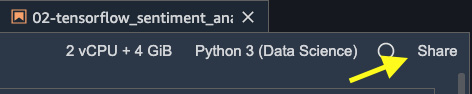
Figure 5.6 – Sharing a notebook in SageMaker Studio with another user
You will be prompted to choose the level of information to be included and will be provided with a URL such as https://<sm-domain-id>.studio.<region>.sagemaker.aws/jupyter/default/lab?sagemaker-share-id=xxxxxxxxxxxxxxxxxxx for anyone who has a user profile in the same SageMaker Studio domain. Once your colleague opens the URL, they will see the read-only notebook, snapshot details, and an option to create a copy to be able to edit the notebook, as shown in Figure 5.7:
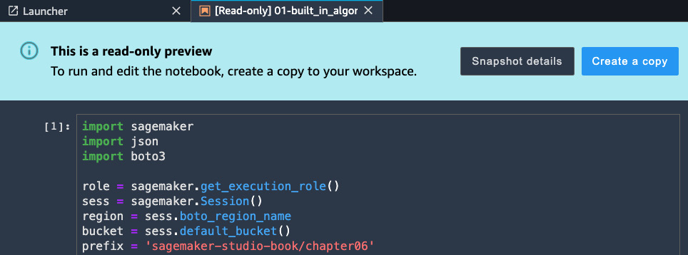
Figure 5.7 – Another user's view of the shared notebook
Note
The notebook-sharing feature requires configuration when the domain is created. Notebook sharing is enabled if you set up the domain using Quickstart, as described in Chapter 2, Introducing Amazon SageMaker Studio. If you use the Standard setup, you need to explicitly enable notebook sharing.
Summary
In this chapter, we explained how you can train a ML model in a notebook in SageMaker Studio. We ran two examples, one using SageMaker's built-in BlazingText algorithm to train a text classification model, and another one using TensorFlow as a deep learning framework to build a network architecture to train a sentiment analysis model to predict the sentiment in movie review data. We learned how SageMaker's fully managed training feature works and how to provision the right amount of compute resources from the SageMaker SDK for your training script.
We demonstrated SageMaker Experiments' ability to manage and compare ML training runs in SageMaker Studio's UI. Besides training with TensorFlow scripts, we also explained how flexible SageMaker training is when working with various ML frameworks, such as PyTorch, MXNet, Hugging Face, and scikit-learn. Last but not least, we showed you how SageMaker's Git integration and notebook-sharing features can help boost your productivity.
In the next chapter, we will learn about SageMaker Clarify and how to apply SageMaker Clarify to detect bias in your data and ML models and to explain how models make decisions. Understanding bias and model explainability is essential to creating a fair ML model. We will dive deep into the approaches, metrics SageMaker Clarify uses to measure the bias and how Clarify explains the model.