6

Working with Date and Time in Python

At the core of time-series data is time. Time-series data is a sequence of observations or data points captured in successive order. In the context of a DataFrame, time-series data has an ordered index type DatetimeIndex as you have seen in earlier chapters.

Being familiar with manipulating date and time in time-series data is an essential component of time series analysis and modeling. In this chapter, you will find recipes for common scenarios when working with date and time in time-series data.

Python has several built-in modules for working with date and time, such as the datetime, time, calendar, and zoneinfo modules. Additionally, there are other popular libraries in Python that further extend the capability to work with and manipulate date and time, such as dateutil, pytz, and arrow, to name a few.

You will be introduced to the datetime module in this chapter but then transition to use pandas for enhanced and more complex date and time manipulation, and generate time-series DataFrames with a sequence of DatetimeIndex. In addition, the pandas library contains several date-specific and time-specific classes that inherit from the aforementioned Python modules. In other words, you will not need to import additional date/time Python libraries.

You will be introduced to pandas classes such as Timestamp, Timedelta, Period, and DateOffset. You will notice similarities between the functionality – for example, the pandas Timestamp class is equivalent to Python's Datetime class and can be interchangeable in most scenarios. Similarly, pandas.Timedelta is equivalent to Python's datetime.timedelta object. The pandas library offers a more straightforward, intuitive, and powerful interface to handle most of your date and time manipulation needs without importing additional modules. When using pandas, you will appreciate having a library that contains everything you need to work with time-series data and can easily handle many challenging tasks.

Here is the list of the recipes that we will cover in this chapter:

• Working with DatetimeIndex
• Providing a format argument to DateTime
• Working with Unix epoch timestamps
• Working with time deltas
• Converting DateTime with time zone information
• Working with date offsets
• Working with custom business days

In a real-world scenario, you may not use all or any of these techniques. Still, it is critical to be aware of the options when facing a particular scenario that requires certain adjustments or formatting of dates.

Technical requirements

In this chapter and going forward, we will extensively use pandas 1.4.2 (released on April 2, 2022. This applies to all the recipes in this chapter.

Load these libraries in advance, since you will be using them throughout the chapter:

import pandas as pd
import numpy as np
import datetime as dt

You will use dt, np, and pd aliases going forward.

You can download the Jupyter notebooks from the GitHub repository at https://github.com/PacktPublishing/Time-Series-Analysis-with-Python-Cookbook./tree/main/code/Ch6 to follow along.

Working with DatetimeIndex

As this ebook edition doesn't have fixed pagination, the page numbers below are hyperlinked for reference only, based on the printed edition of this book.

The pandas library has many options and features to simplify tedious tasks when working with time-series data, dates, and time.

When working with time-series data in Python, it is common to load into a pandas DataFrame with an index of type DatetimeIndex. As an index, the DatetimeIndex class extends pandas DataFrame capabilities to work more efficiently and intelligently with time-series data. This was demonstrated numerous times in Chapter 2, Reading Time Series Data from Files, and Chapter 3, Reading Time Series Data from Databases.

By the end of this recipe, you will appreciate pandas' rich set of date functionality to handle almost any representation of date/time in your data. Additionally, you will learn how to use different functions in pandas to convert date-like objects to a DatetimeIndex.

How to do it…

In this recipe, you will explore Python's datetime module and learn about the Timestamp and DatetimeIndex classes and the relationship between them.

1. To understand the relationship between Python's datetime.datetime class and pandas' Timestamp and DatetimeIndex classes, you will create three different datetime objects representing the date 2021, 1, 1. You will then compare these objects to gain a better understanding:

   dt1 = dt.datetime(2021,1,1)

   dt2 = pd.Timestamp('2021-1-1')

   dt3 = pd.to_datetime('2021-1-1')

Inspect the datetime representation:

print(dt1)
print(dt2)
print(dt3)
>>
2021-01-01 00:00:00
2021-01-01 00:00:00
2021-01-01 00:00:00

Inspect their data types:

print(type(dt1))
print(type(dt2))
print(type(dt3))
>>
<class 'datetime.datetime'>
<class 'pandas._libs.tslibs.timestamps.Timestamp'>
<class 'pandas._libs.tslibs.timestamps.Timestamp'>

And finally, let's see how they compare:

dt1 == dt2 == dt3
>> True
isinstance(dt2, dt.datetime)
>> True    
isinstance(dt2, pd.Timestamp)
>> True
isinstance(dt1, pd.Timestamp)
>> False

You can see from the preceding code that pandas' Timestamp object is equivalent to Python's Datetime object:

issubclass(pd.Timestamp, dt.datetime)
>> True

Note that dt2 is an instance of pandas.Timestamp class, and the Timestamp class is a subclass of Python's dt.datetime class (but not vice versa).

2. When you used the pandas.to_datetime() function, it returned a Timestamp object. Now, use pandas.to_datetime() on a list and examine the outcome:

   dates = ['2021-1-1', '2021-1-2']

   pd_dates = pd.to_datetime(dates)

   print(pd_dates)

   print(type(pd_dates))

   >>

   DatetimeIndex(['2021-01-01', '2021-01-02'], dtype='datetime64[ns]', freq=None)

   <class 'pandas.core.indexes.datetimes.DatetimeIndex'>

Interestingly, the output is now of type DatetimeIndex created using the same pandas.to_datetime() function that you used earlier. Previously, when using the same function on an individual object, the result was of type Timestamp, but when applied on a list, it produced a sequence of type DatetimeIndex. You will perform one more task to make things clearer.

Print out the first item (slice) from the pd_dates variable:

print(pd_dates[0])
print(type(pd_dates[0]))
>> 
2021-01-01 00:00:00
<class 'pandas._libs.tslibs.timestamps.Timestamp'>

From the preceding output, you can infer a relationship between the two classes: DatetimeIndex and Timestamp. A DatetimeIndex is a sequence (list) of Timestamp objects.

3. Now that you know how to create a DatetimeIndex using the pandas.to_datetime() function, let's further expand on this and see what else you can do with the function. For example, you will see how simple it is to convert different datetime representations, including strings, integers, lists, pandas series, or other datetime objects, into a DatetimeIndex.

Let's create a dates list:

dates = ['2021-01-01', 
         '2/1/2021', 
         '03-01-2021', 
         'April 1, 2021', 
         '20210501', 
          np.datetime64('2021-07-01'), # numpy datetime64
          datetime.datetime(2021, 8, 1), # python datetime
          pd.Timestamp(2021,9,1) # pandas Timestamp
          ]

Parse the list using pandas.to_datetime():

parsed_dates = pd.to_datetime(
                 dates,
                 infer_datetime_format=True,
                 errors='coerce'
                 )
print(parsed_dates)
>>
DatetimeIndex(['2021-01-01', '2021-02-01', '2021-03-01', '2021-04-01', '2021-05-01', '2021-07-01', '2021-08-01', '2021-09-01'],
              dtype='datetime64[ns]', freq=None)

Notice how the that the to_datetime() function properly parsed the entire list of different string representations and date types such as Python's Datetime and NumPy's datetime64. Similarly, you could have used the DatetimeIndex constructor directly, as follows:

pd.DatetimeIndex(dates)

This would produce similar results.

4. The DatetimeIndex object gives access to many useful properties and methods to extract additional date and time properties. As an example, you can extract day_name, month, year, days_in_month, quarter, is_quarter_start, is_leap_year, is_month_start, is_month_end, and is_year_start. The following code shows how this can be done:

   print(f'Name of Day : {parsed_dates.day_name()}')

   print(f'Month : {parsed_dates.month}')

   print(f'Year : {parsed_dates.year}')

   print(f'Days in Month : {parsed_dates.days_in_month}')

   print(f'Quarter {parsed_dates.quarter}')

   print(f'Quarter Start : {parsed_dates.is_quarter_start}')

   print(f'Leap Year : {parsed_dates.is_leap_year}')

   print(f'Month Start : {parsed_dates.is_month_start}')

   print(f'Month End : {parsed_dates.is_month_end}')

   print(f'Year Start : {parsed_dates.is_year_start}')

The preceding code produces the following results:

Name of Day : Index(['Friday', 'Monday', 'Monday', 'Thursday',   
                'Saturday', 'Thursday', Sunday', 'Wednesday'],
                  dtype='object')
Month : Int64Index([1, 2, 3, 4, 5, 7, 8, 9], dtype='int64')
Year : Int64Index([2021, 2021, 2021, 2021, 2021, 2021, 2021, 2021], dtype='int64')
Days in Month : Int64Index([31, 28, 31, 30, 31, 31, 31, 30], dtype='int64')
Quarter Int64Index([1, 1, 1, 2, 2, 3, 3, 3], dtype='int64')
Quarter Start : [ True False False  True False  True False False]
Leap Year : [False False False False False False False False]
Month Start : [ True  True  True  True  True  True  True  True]
Month End : [False False False False False False False False]
Year Start : [ True False False False False False False False]

These properties and methods will be very useful when transforming your time-series datasets for analysis.

How it works…

The, pandas.to_datetime() is a powerful function that can intelligently parse different date representations from strings. As you saw in step 4 in the previous How to do it… section, the string examples, such as '2021-01-01', '2/1/2021', '03-01-2021', 'April 1, 2021', and '20210501', were parsed correctly. Other date representations such as 'April 1, 2021' and '1 April 2021', can be parsed using the to_datetime() function as well, and I'll leave it to you to explore additional examples that come to mind.

The to_datetime function contains the errors parameter. In the following example, you specify errors='coerce' which instructs pandas to set any value it could not parse as NaT indicating a missing value. You will learn more about NaT in the Performing data quality checks recipe in Chapter 7, Handling Missing Data.

pd.to_datetime(
                 dates,
                 infer_datetime_format=True,
                 errors='coerce'
                 )

In pandas, there are different representations to indicate missing values – np.NaN represents missing numeric values (Not a Number), while pd.NaT represents missing datetime values (Not a Time). Finally, pandas' pd.NA is used to represent missing scalar values (Not Available).

The errors parameter in to_datetime can take one of the three valid string options:

• raise, which means it will raise an exception (error out).
• coerce will not cause it to raise an exception. Instead, it will just replace pd.NaT, indicating a missing datetime value.
• ignore will also not cause it to raise an exception. Instead, it will just pass in the original value.

Here is an example using the ignore value:

pd.to_datetime(['something 2021', 'Jan 1, 2021'], 
               errors='ignore')
>> Index(['something 2021', 'Jan 1, 2021'], dtype='object')

When the errors parameter is set to 'ignore', pandas will not raise an error if it stumbles upon a date representation it cannot parse. Instead, the input value is passed as-is. For example, notice from the preceding output that the to_datetime function returned an Index type and not a DatetimeIndex. Further, the items in the Index sequence are of dtype object (and not datetime64). In pandas, the object dtype represents strings or mixed types.

There's more…

An alternate way to generate a of DatetimeIndex is with the pandas.date_range() function. The following code provides a starting date and the number of periods to generate and specifies a daily frequency with D:

pd.date_range(start='2021-01-01', periods=3, freq='D')
>>
DatetimeIndex(['2021-01-01', '2021-01-02', '2021-01-03'], dtype='datetime64[ns]', freq='D')

pandas.date_range() requires at least three of the four parameters to be provided – start, end, periods, and freq. If you do not provide enough information, you will get a ValueError exception with the following message:

ValueError: Of the four parameters: start, end, periods, and freq, exactly three must be specified

Let's explore the different parameter combinations required to use the date_range function. In the first example, provide a start date, end date, and specify a daily frequency. The function will always return a range of equally spaced time points:

pd.date_range(start='2021-01-01',
               end='2021-01-03',
               freq='D')
>>
DatetimeIndex(['2021-01-01', '2021-01-02', '2021-01-03'], dtype='datetime64[ns]', freq='D')

In the second example, provide a start date and an end date, but instead of frequency, provide a number of periods. Remember that the function will always return a range of equally spaced time points:

pd.date_range(start='2021-01-01',
               end='2021-01-03',
               periods=2)
>>
DatetimeIndex(['2021-01-01', '2021-01-03'], dtype='datetime64[ns]', freq=None)
pd.date_range(start='2021-01-01',
               end='2021-01-03',
               periods=4)
>>
DatetimeIndex(['2021-01-01 00:00:00', '2021-01-01 16:00:00',
               '2021-01-02 08:00:00', '2021-01-03 00:00:00'],
              dtype='datetime64[ns]', freq=None)

In the following example, provide an end date and the number of periods returned, and indicate a daily frequency:

pd.date_range(end='2021-01-01', periods=3, freq='D')
DatetimeIndex(['2020-12-30', '2020-12-31', '2021-01-01'], dtype='datetime64[ns]', freq='D')

Note, the pd.date_range() function can work with a minimum of two parameters if the information is sufficient to generate equally spaced time points and infer the missing parameters. Here is an example of providing start and end dates only:

pd.date_range(start='2021-01-01',
               end='2021-01-03')
>>
DatetimeIndex(['2021-01-01', '2021-01-02', '2021-01-03'], dtype='datetime64[ns]', freq='D')

Notice that pandas was able to construct the date sequence using the start and end dates and default to daily frequency. Here is another example:

pd.date_range(start='2021-01-01',
               periods=3)
>>
DatetimeIndex(['2021-01-01', '2021-01-02', '2021-01-03'], dtype='datetime64[ns]', freq='D')

With start and periods, pandas has enough information to construct the date sequence and default to daily frequency.

Now, here is an example that lacks enough information on how to generate the sequence and will cause pandas to throw an error:

pd.date_range(start='2021-01-01',
               freq='D')
>>
ValueError: Of the four parameters: start, end, periods, and freq, exactly three must be specified

Note that with just a start date and frequency, pandas does not have enough information to construct the date sequence. Therefore, adding either periods or the end date will be sufficient.

See also

To learn more about pandas' to_datetime() function and the DatetimeIndex class, please check out these resources:

• pandas.DatetimeIndex documentation: https://pandas.pydata.org/docs/reference/api/pandas.DatetimeIndex.html
• pandas.to_datetime documentation: https://pandas.pydata.org/docs/reference/api/pandas.to_datetime.html

Providing a format argument to DateTime

When working with datasets extracted from different data sources, you may encounter date columns stored in string format, whether from files or databases. In the previous recipe, Working with DatetimeIndex, you explored the pandas.to_datetime() function that can parse various date formats with minimal input. However, you will want more granular control to ensure that the date is parsed correctly. For example, you will now be introduced to the strptime and strftime methods and see how you can specify formatting in pandas.to_datetime() to handle different date formats.

In this recipe, you will learn how to parse strings that represent dates to a datetime or date object (an instance of the class datetime.datetime or datetime.date).

How to do it…

Python's datetime module contains the strptime() method to create datetime or date from a string that contains a date. You will first explore how you can do this in Python and then extend this to pandas:

1. Let's explore a few examples, parsing strings to datetime objects using datetime.strptime. You will parse four different representations of January 1, 2022 that will produce the same output – datetime.datetime(2022, 1, 1, 0, 0):

   dt.datetime.strptime('1/1/2022', '%m/%d/%Y')

   dt.datetime.strptime('1 January, 2022', '%d %B, %Y')

   dt.datetime.strptime('1-Jan-2022', '%d-%b-%Y')

   dt.datetime.strptime('Saturday, January 1, 2022', '%A, %B %d, %Y')

   >>

   datetime.datetime(2022, 1, 1, 0, 0)

Note that the output is a datetime object, representing the year, month, day, hour, and minute. You can specify only the date representation, as follows:

dt.datetime.strptime('1/1/2022', '%m/%d/%Y').date()
>>
datetime.date(2022, 1, 1)

Now, you will have a date object instead of datetime. You can get the readable version of datetime using the print() function:

dt_1 = dt.datetime.strptime('1/1/2022', '%m/%d/%Y')
print(dt_1)
>>
2022-01-01 00:00:00

2. Now, let's compare what you did using the datetime.strptime method using pandas.to_datetime method:

   pd.to_datetime('1/1/2022', format='%m/%d/%Y')

   pd.to_datetime('1 January, 2022', format='%d %B, %Y')

   pd.to_datetime('1-Jan-2022', format='%d-%b-%Y')

   pd.to_datetime('Saturday, January 1, 2022', format='%A, %B %d, %Y')

   >>

   Timestamp('2022-01-01 00:00:00')

Similarly, you can get the string (readable) representation of the Timestamp object using the print() function:

dt_2 = pd.to_datetime('1/1/2022', format='%m/%d/%Y')
print(dt_2)
>> 
2022-01-01 00:00:00

3. There is an advantage in using pandas.to_datetime() over Python's datetime module. The to_datetime() function can parse a variety of date representations, including string date formats with minimal input or specifications. The following code explains this concept; note that the format is omitted:

   pd.to_datetime('Saturday, January 1, 2022')

   pd.to_datetime('1-Jan-2022')

   >> 

   Timestamp('2022-01-01 00:00:00')

Note that unlike datetime, which requires integer values or to use the strptime method for parsing strings, the pandas.to_datetime() function can intelligently parse different date representations without specifying a format (this is true in most cases).

How it works…

In this recipe, you used Python's datetime.datetime and pandas.to_datetime methods to parse dates in string formats. When using datetime, you had to use the dt.datetime.strptime() function to specify the date format representation in the string using format codes (example %d, %B, and %Y).

For example, in datetime.strptime('1 January, 2022', '%d %B, %Y'), you provided the %d, %B, and %Y format codes in the exact order and spacing to represent the formatting provided in the string. Let's break this down:

Figure 6.1 – Understanding the format

• %d indicates that the first value is a zero-padded digit representing the day of the month, followed by a space to display spacing between the digit and the next object.
• %B is used to indicate that the second value represents the month's full name. Note that this was followed by a comma (,) to describe the exact format in the string, for example "January,". Therefore, it is crucial to match the format in the strings you are parsing to include any commas, hyphens, backslashes, spaces, or whichever separator characters are used.
• To adhere to the string format, there is a space after the comma (,), followed by %Y to reflect the last value represents a four-digit year.

  Format Directives

  Remember that you always use the percent sign (%) followed by the format code (a letter with or without a negative sign). This is called a formatting directive. For example, lower case y, as in %y, represents the year 22 without the century, while uppercase y, as in %Y, represents the year 2022 with the century. Here is a list of common Python directives that can be used in the strptime() function: https://docs.python.org/3/library/datetime.html#strftime-and-strptime-format-codes.

Recall that you used pandas.to_datetime() to parse the same string objects as with dt.datetime.strptime(). The biggest difference is that the pandas function can accurately parse the strings without explicitly providing an argument to the format parameter. That is one of many advantages of using pandas for time-series analysis, especially when handling complex date and datetime scenarios.

There's more…

Now you know how to use pandas.to_datetime() to parse string objects to datetime. So, let's see how you can apply this knowledge to transform a DataFrame column that contains date information in string format to a datetime data type.

In the following code, you will create a small DataFrame:

df = pd.DataFrame(
        {'Date': ['January 1, 2022', 'January 2, 2022', 'January 3, 2022'],
         'Sales': [23000, 19020, 21000]}
            )
df
>>
Date  Sales
0     January 1, 2022   23000
1     January 2, 2022   19020
2     January 3, 2022   21000
df.info()
>>
<class 'pandas.core.frame.DataFrame'>
RangeIndex: 3 entries, 0 to 2
Data columns (total 2 columns):
 #   Column  Non-Null Count  Dtype 
---  ------  --------------  ----- 
 0   Date    3 non-null      object
 1   Sales   3 non-null      int64 
dtypes: int64(1), object(1)
memory usage: 176.0+ bytes

To update the DataFrame to include a DatetimeIndex, you will parse the Date column to datetime and then assign it as an index to the DataFrame:

df['Date'] = pd.to_datetime(df['Date'])
df.set_index('Date', inplace=True)
df.info()
>>
<class 'pandas.core.frame.DataFrame'>
DatetimeIndex: 3 entries, 2022-01-01 to 2022-01-03
Data columns (total 1 columns):
 #   Column  Non-Null Count  Dtype
---  ------  --------------  -----
 0   Sales   3 non-null      int64
dtypes: int64(1)
memory usage: 48.0 bytes

Note how the index is now of the DatetimeIndex type, and there is only one column in the DataFrame (Sales), since Date is now an index.

See also

To learn more about pandas.to_datetime, please visit the official documentation page here: https://pandas.pydata.org/docs/reference/api/pandas.to_datetime.html.

Working with Unix epoch timestamps

Epoch timestamps, sometimes referred to as Unix time or POSIX time, are a common way to store datetime in an integer format. This integer represents the number of seconds elapsed from a reference point, and in the case of a Unix-based timestamp, the reference point is January 1, 1970, at midnight (00:00:00 UTC). This arbitrary date and time represent the baseline, starting at 0. So, we just increment in seconds for every second beyond that time.

Many databases, applications, and systems store dates and time in numeric format, making it mathematically easier to work with, convert, increment, decrement, and so on. Note that in the case of the Unix epoch, it is based on UTC, which stands for Universal Time Coordinated. Using UTC is a clear choice when building applications used globally, making it easier to store dates and timestamps in a standardized format. This makes it easier to work with dates and time without worrying about daylight saving or different time zones around the globe. UTC is the standard international time used in aviation systems, weather forecast systems, the International Space Station, and so on.

You will, at some point, encounter Unix epoch timestamps, and to make more sense of the data, you will need to convert it to a human-readable format. This is what will be covered in this recipe. Again, you will explore the ease of using pandas' built-in functions to work with Unix epoch timestamps.

How to do it…

Before we start converting the Unix time to a human-readable datetime object, which is the easy part, let's first gain some intuition about the idea of storing dates and time as a numeric object (a floating-point number):

1. You will use time from the time module (part of Python) to request the current time in seconds. This will be the time in seconds since the epoch, which for Unix systems starts from January 1, 1970, at 00:00:00 UTC:

   import time

   epoch_time = time.time()

   print(epoch_time)

   print(type(epoch_time))

   >>

   1635220133.855169

   <class 'float'>
2. Now, copy the numeric value you have and visit https://www.epoch101.com. The website should display your current epoch time. If you scroll down, you can paste the number and convert it to a human-readable format. Make sure that you click on seconds, as shown in the following figure:

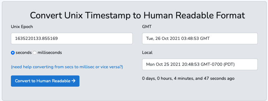
Figure 6.2 – Converting a Unix timestamp to a human-readable format in both GMT and local time

Note, the GMT format was given as Tue, 26 Oct 2021 03:48:53 GMT and my local format as Mon Oct 25, 2021, 20:48:53 GMT-0700 (PDT).

3. Let's see how pandas converts the epoch timestamp. The convenience here is that you will be using the same pandas.to_datetime() function that you should be familiar with by now, as you have used it in the previous two recipes from this chapter. This is one of the many conveniences you get when using pandas. For example, in the following code, you will use pandas.to_datetime() to parse the Unix epoch 1635220133.855169:

   import pandas as pd

   t = pd.to_datetime(1635220133.855169, unit='s')

   print(t)

   >>

   2021-10-26 03:48:53.855169024

Note the need to specify units as seconds. The output is similar to that in Figure 6.1 for the GMT format.

4. If you want datetime to be time-zone aware – for example, the US/Pacific time zone – you can use tz_localize('US/Pacific'). To get a more accurate conversion though, it is better to do it in two steps:
   1. Convert the time zone-naive object to UTC using tz_localize('UTC').
   2. Then, convert it to the desired time zone using tz_convert().

The following code shows how this is done to convert to the Pacific time zone:

t.tz_localize('UTC').tz_convert('US/Pacific')
>>
Timestamp('2021-10-25 20:48:53.855169024-0700', tz='US/Pacific')

Compare this to Figure 6.1 for the local Pacific Daylight Time (PDT) format, and it will be the same.

5. Let's put all of this together. You will convert a DataFrame that contains a datetime column in Unix epoch format to a human-readable format. You will start by creating a new DataFrame with Unix epoch timestamps:

   df = pd.DataFrame(

           {'unix_epoch': [1641110340,  1641196740, 1641283140, 1641369540],

                   'Sales': [23000, 19020, 21000, 17030]}

                   )

   df

   >>

         unix_epoch  Sales

   0     1641110340  23000

   1     1641196740  19020

   2     1641283140  21000

   3     1641369540  17030
6. Create a new column, call it Date by parsing the unix_epoch column into a datetime (which defaults to GMT), then localize the output to UTC, and convert to a local time zone. Finally, set the Date column as the index:

   df['Date'] = pd.to_datetime(df['unix_epoch'], unit='s')

   df['Date'] = df['Date'].dt.tz_localize('UTC').dt.tz_convert('US/Pacific')

   df.set_index('Date', inplace=True)

   df

   >>                              unix_epoch  Sales

   Date        

   2022-01-01 23:59:00-08:00     1641110340  23000

   2022-01-02 23:59:00-08:00     1641196740  19020

   2022-01-03 23:59:00-08:00     1641283140  21000

   2022-01-04 23:59:00-08:00     1641369540  17030

Note that since the Date column was of the datetime type (not DatetimeIndex), you had to use the Series.dt accessor to tap into the built-in methods and attributes for the datetime objects. In the last step, you converted datetime to a DatetimeIndex object (a DataFrame index). If you recall from the Working with DatetimeIndex recipe of this chapter, a DatetimeIndex object can access any of the datetime methods and attributes without using the dt accessor.

7. If you do not need the time in your index (DatetimeIndex), given your data is daily and there is no use case for using time, then you can request just the date, as shown in the following code:

   df.index.date

   >>

   array([datetime.date(2022, 1, 1), datetime.date(2022, 1, 2), datetime.date(2022, 1, 3), datetime.date(2022, 1, 4)], dtype=object)

Note that the output displays the date without time.

How it works…

So far, you have used pandas.to_datetime() to parse dates in string format to a datetime object by leveraging the format attribute (see the Providing a format argument to DateTime recipe). In this recipe, you used the same function, but instead of providing a value to format, you passed a value to the unit parameter, as in unit="s." .

The unit parameter tells pandas which unit to use when calculating the difference from the epoch start. In this case, the request was in seconds. However, there is another critical parameter that you do not need to adjust (in most cases), which is the origin parameter. For example, the default value is origin='unix', which indicates that the calculation should be based on the Unix (or POSIX) time set to 01-01-1970 00:00:00 UTC.

This is what the actual code looks like:

pd.to_datetime(1635220133.855169, unit='s', origin='unix')
>>
Timestamp('2021-10-26 03:48:53.855169024')

There's more…

If you would like to store your datetime value in Unix epoch, you can do this by subtracting 1970-01-01 and then floor-divide by a unit of 1 second. Python uses / as the division operator, // as the floor division operator to return the floored quotient, and % as the modulus operator to return the remainder from a division.

Start by creating a new pandas DataFrame:

df = pd.DataFrame(
        {'Date': pd.date_range('01-01-2022', periods=5),
        'order' : range(5)}
                 )
df
>>
      Date        order
0     2022-01-01    0
1     2022-01-02    1
2     2022-01-03    2
3     2022-01-04    3
4     2022-01-05    4

You can then perform the transformation, as follows:

(df['Date'] -  pd.Timestamp("1970-01-01")) // pd.Timedelta("1s")
>>
0    1640995200
1    1641081600
2    1641168000
3    1641254400
4    1641340800

You have now generated your Unix epochs. There are different ways to achieve similar results. The preceding example is the recommended approach from pandas, which you can read more about here: https://pandas.pydata.org/pandas-docs/stable/user_guide/timeseries.html#from-timestamps-to-epoch.

See also

To learn more about pandas.to_datetime, please visit the official documentation page here: https://pandas.pydata.org/docs/reference/api/pandas.to_datetime.html.

Working with time deltas

When working with time-series data, you may need to perform some calculations on your datetime columns, such as adding or subtracting. Examples can include adding 30 days to purchase datetime to determine when the return policy expires for a product or when a warranty ends. For example, the Timedelta class makes it possible to derive new datetime objects by adding or subtracting at different ranges or increments, such as seconds, daily, and weekly. This includes time zone-aware calculations.

In this recipe, you will explore two practical approaches in pandas to capture date/time differences – the pandas.Timedelta class and the pandas.to_timedelta function.

How to do it…

In this recipe, you will work with hypothetical sales data for a retail store. You will generate the sales DataFrame, which will contain items purchased from the store and the purchase date. You will then explore different scenarios using the Timedelta class and the to_timedelta() function:

1. Start by importing the pandas library and creating a DataFrame with two columns, item and purchase_dt, which will be standardized to UTC:

   df = pd.DataFrame(

           {       

           'item': ['item1', 'item2', 'item3', 'item4', 'item5', 'item6'],

           'purchase_dt': pd.date_range('2021-01-01', periods=6, freq='D', tz='UTC')

           }

   )

   df

The preceding code should output a DataFrame with six rows (items) and two columns (item and purchase_dt):

Figure 6.3 – The DataFrame with the item purchased and purchase datetime (UTC) data

2. Add another datetime column to represent the expiration date, which is 30 days from the purchase date:

   df['expiration_dt'] = df['purchase_dt'] + pd.Timedelta(days=30)

   df

The preceding code should add a third column (expiration_dt) to the DataFrame, which is set at 30 days from the date of purchase:

Figure 6.4 – The updated DataFrame with a third column reflecting the expiration date

3. Now, assume you are asked to create a special extended date for return, and this one is set at 35 days, 12 hours, and 30 minutes from the purchase date:

   df['extended_dt'] = df['purchase_dt'] +

                   pd.Timedelta('35 days 12 hours 30 minutes')

   df

The preceding code should add a fourth column (extended_dt) to the DataFrame, reflecting the new datetime, based on the additional 35 days, 12 hours, and 30 minutes:

Figure 6.5 – The updated DataFrame with a fourth datetime column reflecting the extended date

4. Assume that you are asked to convert the time zone from UTC to the local time zone of the retailer store's headquarters, which is set in Los Angeles:

   df.iloc[:,1:] = df.iloc[: ,1:].apply(

               lambda x: x.dt.tz_convert('US/Pacific')

                   )

   df

After converting from UTC to the US/Pacific time zone (Los Angeles), you are overwriting the datetime columns (purchased_dt, expiration_dt, and extended_dt). The DataFrame structure should remain the same – six rows and four columns – but now the data looks different, as shown in the following screenshot:

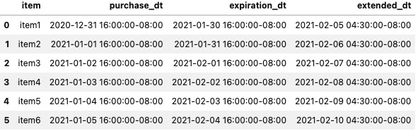
Figure 6.6 – The updated DataFrame where all datetime columns are in Los Angeles (US/Pacific)

5. Finally, you can calculate the delta between the extended and original expiration dates. Since they are both datetime data types, you can achieve this with a simple subtraction between the two columns:

   df['exp_ext_diff'] = (

            df['extended_dt'] - df['expiration_dt']

           )

   df

Your final DataFrame should now have a fifth column that captures the difference between the extended date and the expiration date:

Figure 6.7 – The updated DataFrame with a fifth column

These types of transformations and calculations are simplified without needing any additional libraries, thanks to pandas' built-in capabilities to work with time-series data and datetime overall.

How it works…

Time deltas can be handy for capturing the difference between two date or time objects. In pandas, the pandas.Timedelta class is equivalent to Python's datetime.timedelta class and behaves very similarly. However, the advantage of pandas is that it includes a wide range of classes and functions for working with time-series data. These built-in functions within pandas, in general, are simpler and more efficient when working with DataFrames. Let's try this quick experiment to demonstrate how pandas' Timedelta class is a subclass of Python's timedelta class:

import datetime as dt
import pandas as pd
pd.Timedelta(days=1) == dt.timedelta(days=1)
>> True

Let's validate that pandas.Timedelta is an instance of datetime.timedelta:

issubclass(pd.Timedelta, dt.timedelta)
>> True
dt_1 = pd.Timedelta(days=1)
dt_2 = dt.timedelta(days=1)
isinstance(dt_1, dt.timedelta)
>> True
isinstance(dt_1, pd.Timedelta)
>> True

Python's datetime.timedelta class accepts integer values for these parameters – days, seconds, microseconds, milliseconds, minutes, hours, and weeks. On the other hand, pandas.Timedelta takes both integers and strings, as demonstrated in the following snippet:

pd.Timedelta(days=1, hours=12, minutes=55)
>> Timedelta('1 days 12:55:00')
pd.Timedelta('1 day 12 hours 55 minutes')
>> Timedelta('1 days 12:55:00')
pd.Timedelta('1D 12H 55T')
>> Timedelta('1 days 12:55:00')

Once you have defined your Timedelta object, you can use it to make calculations on date, time, or datetime objects:

week_td = pd.Timedelta('1W')
pd.to_datetime('1 JAN 2022') + week_td
>> Timestamp('2022-01-08 00:00:00')

In the preceding example, week_td represents a 1-week Timedelta object, which can be added (or subtracted) from datetime to get the difference. By adding week_td, you are incrementing by 1 week. What if you want to add 2 weeks? You can use multiplication as well:

pd.to_datetime('1 JAN 2022') + 2*week_td
>> Timestamp('2022-01-15 00:00:00')

There's more…

Using pd.Timedelta is straightforward and makes working with large time-series DataFrames efficient without importing additional libraries, as it is built into pandas.

In the previous How to do it... section, you created a DataFrame and added additional columns based on the timedelta calculations. You can also add the timedelta object into a DataFrame and reference it by its column. Finally, let's see how this works.

First, let's construct the same DataFrame used earlier:

import pandas as pd
df = pd.DataFrame(
        {       
        'item': ['item1', 'item2', 'item3', 'item4', 'item5', 'item6'],
        'purchase_dt': pd.date_range('2021-01-01', periods=6, freq='D', tz='UTC')
        }
)

This should print out the DataFrame shown in Figure 6.2. Now, you will add a new column that contains the Timedelta object (1 week) and then use that column to add and subtract from the purchased_dt column:

df['1 week'] = pd.Timedelta('1W')
df['1_week_more'] = df['purchase_dt'] + df['1 week']
df['1_week_less'] = df['purchase_dt'] - df['1 week']
df

The preceding code should produce a DataFrame with three additional columns. The 1 week column holds the Timedelta, object and because of that, you can reference the column to calculate any time differences you need:

Figure 6.8 – The updated DataFrame with three additional columns

Let's check the data types for each column in the DataFrame:

df.info()
>>
<class 'pandas.core.frame.DataFrame'>
RangeIndex: 6 entries, 0 to 5
Data columns (total 5 columns):
 #   Column       Non-Null Count  Dtype              
---  ------       --------------  -----              
 0   item         6 non-null      object             
 1   purchase_dt  6 non-null      datetime64[ns, UTC]
 2   1 week       6 non-null      timedelta64[ns]    
 3   1_week_more  6 non-null      datetime64[ns, UTC]
 4   1_week_less  6 non-null      datetime64[ns, UTC]
dtypes: datetime64[ns, UTC](3), object(1), timedelta64[ns](1)
memory usage: 368.0+ bytes

Note that the 1 week column is a particular data type, timedelta64 (our Timedelta object), which allows you to make arithmetic operations on the date, time, and datetime columns in your DataFrame.

In the Working with DatetimeIndex recipe, you explored the pandas.date_range() function to generate a DataFrame with DatetimeIndex. The function returns a range of equally spaced time points based on the start, end, period and frequency parameters.

Similarly, you have an option to generate TimdedeltaIndex with a fixed frequency using the pandas.timedelta_range() function, which takes similar parameters as the pandas.date_range() function. Here is a quick example:

df = pd.DataFrame(
        {       
        'item': ['item1', 'item2', 'item3', 'item4', 'item5'],
        'purchase_dt': pd.date_range('2021-01-01', periods=5, freq='D', tz='UTC'),
        'time_deltas': pd.timedelta_range('1W 2 days 6 hours', periods=5)
        }
)
df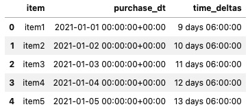

The output is as follows:

Figure 6.9 – A DataFrame with a Timedelta column

See also

• To learn more about the pandas.timedelta_range() function, please refer to the official documentation here: https://pandas.pydata.org/docs/reference/api/pandas.timedelta_range.html.
• To learn more about the pandas.Timedelta class, please visit the official documentation here: https://pandas.pydata.org/docs/reference/api/pandas.Timedelta.html.

Converting DateTime with time zone information

When working with time-series data that requires attention to different time zones, things can get out of hand and become more complicated. For example, when developing data pipelines, building a data warehouse, or integrating data between systems, dealing with time zones requires attention and consensus amongst the different stakeholders in the project. For example, in Python, there are several libraries and modules dedicated to working with time zone conversion; these include pytz, dateutil, and zoneinfo, to name a few.

Let's discuss an inspiring example regarding time zones within time-series data. It is common for large companies that span their products and services across continents to include data from different places around the globe. For example, it would be hard to make data-driven business decisions if we neglect time zones. Let's say you want to determine whether most customers come to your e-commerce site in the morning or evening, and whether shoppers browse during the day and then make a purchase in the evening after work. For this analysis, you need to be aware of time zone differences and their interpretation on an international scale.

How to do it…

In this recipe, you will work with a hypothetical scenario – a small dataset that you will generate to represent website visits at different time intervals from various locations worldwide. The data will be standardized to UTC, and you will work with time-zone conversions.

1. You will start by importing the pandas library and creating the time-series DataFrame:

   df = pd.DataFrame(

           {       

           'Location': ['Los Angeles', 

                        'New York',

                        'Berlin', 

                        'New Delhi', 

                        'Moscow', 

                        'Tokyo', 

                        'Dubai'],

           'tz': ['US/Pacific', 

                  'US/Eastern', 

                  'Europe/Berlin', 

                  'Asia/Kolkata', 

                  'Europe/Moscow', 

                  'Asia/Tokyo',

                  'Asia/Dubai'],

           'visit_dt': pd.date_range(start='22:00',periods=7, freq='45min'),

           }).set_index('visit_dt')

   df

This will produce a DataFrame where visit_dt is the index of the DatetimeIndex type and two columns, Location and tz, indicate the time zone:

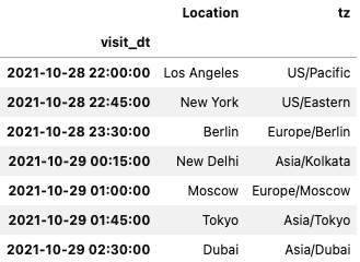
Figure 6.10 – The DataFrame with visit_dt in UTC as an index

2. Assume that you need to convert this DataFrame to be in the same time zone as the company's headquarters in Tokyo. You can do this easily using DataFrame.tz_convert() against the DataFrame, but you will get a TypeError exception if you do this. That is because your time-series DataFrame is not time zone-aware. So, you need to localize it first using tz_localize() to make it time-zone aware. In this case, you will localize it to UTC:

   df = df.tz_localize('UTC')
3. You will now convert the DataFrame to the headquarters' time zone (Tokyo):

   df_hq = df.tz_convert('Asia/Tokyo')

   df_hq

The DataFrame index, visit_dt, will be converted to the new time zone:

Figure 6.11 – The DataFrame index converted to the headquarters' time zone (Tokyo)

Note that you were able to access the tz_localize() and tz_convert() methods because the DataFrame had an index of type DatetimeIndex. If that was not the case, you would get a TypeError exception with the following message:

TypeError: index is not a valid DatetimeIndex or PeriodIndex 

4. Now, you will localize each row to the appropriate time zone. You will add a new column reflecting the time zone, based on the location of the user that accessed the website. You will leverage the tz column to accomplish this:

   df['local_dt'] = df.index

   df['local_dt'] = df.apply(lambda x: pd.Timestamp.tz_convert(x['local_dt'], x['tz']), axis=1)

   df

This should produce a new column, local_dt, which is based on the UTC datetime from visit_dt and converted based on the time zone provided in the tz column:

Figure 6.12 – The updated DataFrame with local_dt based on a localized time zone for each visit

You may wonder, what if you did not have a tz column? Where would you find the right tz string? Well, these are called Time Zone (TZ) database names. These are standard names, and you can find a subset of these in the Python documentation, or for a more comprehensive list, you can visit this link: https://en.wikipedia.org/wiki/List_of_tz_database_time_zones.

How it works…

Converting a time-series DataFrame from one time zone to another was achieved using DataFrame.tz_convert(), providing it with a time-zone string argument such as US/Pacific. There are a few assumptions when using DataFrame.tz_convert() that you need to keep in mind:

• The DataFrame should have an index of the DatetimeIndex type.
• DatetimeIndex needs to be time zone-aware.

You used the DataFrame.tz_localize() function to make the index time zone aware. It is a good practice to standardize on UTC if you are dealing with different time zones and daylight saving, since UTC is always consistent and never changes (regardless of where you are or if daylight saving time is applied or not). Once in UTC, converting to other time zones is very straightforward.

We first localized the data in the previous steps and then converted it to a different time zone in two steps. You can also do this in one step by chaining the two methods, as shown in the following code:

df.tz_localize('UTC').tz_convert('Asia/Tokyo')

If your index is already time zone-aware, then using tz_localize() will produce a TypeError exception with the following message:

TypeError: Already tz-aware, use tz_convert to convert

This indicates that you do not need to localize it again. Instead, just convert it to another time zone.

There's more…

Looking at the DataFrame in Figure 6.11, it is hard to tell immediately whether the time was in the morning (AM) or evening (PM). You can format datetime using strftime (which we discussed in the Providing a format argument to DateTime recipe).

You will construct the same DataFrame, localize it to UTC, then convert it to the headquarters' time zone, and apply the new format:

df = pd.DataFrame(
        {       
        'Location': ['Los Angeles', 
                     'New York',
                     'Berlin', 
                     'New Delhi', 
                     'Moscow', 
                     'Tokyo', 
                     'Dubai'],
        'tz': ['US/Pacific', 
               'US/Eastern', 
               'Europe/Berlin', 
               'Asia/Kolkata', 
               'Europe/Moscow', 
               'Asia/Tokyo',
               'Asia/Dubai'],
        'visit_dt': pd.date_range(start='22:00',periods=7, freq='45min'),
        }).set_index('visit_dt').tz_localize('UTC').tz_convert('Asia/Tokyo')

We have combined the steps, and this should produce a DataFrame similar to the one in Figure 6.11.

Now, you can update the formatting to use the pattern – YYYY-MM-DD HH:MM AM/PM:

df.index = df.index.strftime('%Y-%m-%d %H:%M %p')
df

The index will be updated from a format/layout perspective. However, it is still time zone-aware, based on Tokyo's time zone, and the index is still DatetimeIndex. The only change is to the datetime layout:

Figure 6.13 – The updated DataFrame index, formatted based on the date format string provided

I am sure you will agree that this is easier to present to users to determine whether the visit was AM or PM quickly.

See also

To learn more about tz_convert you can read the official documentation at https://pandas.pydata.org/docs/reference/api/pandas.Series.dt.tz_convert.html and https://pandas.pydata.org/docs/reference/api/pandas.Timestamp.tz_convert.html.

Working with date offsets

When working with time series, it is critical that you learn more about the data you are working with and how it relates to the problem you are attempting to solve. For example, when working with manufacturing or sales data, you cannot assume that an organization's working day is Monday to Friday or whether it uses the standard calendar year or fiscal year. You should also consider understanding any holiday schedule, annual shutdowns, and other matters related to the business operation.

This is where offsets can be handy. They can help transform your dates into something more meaningful and relatable to a business. They can also help correct data entries that may not be logical.

We will work through a hypothetical example in this recipe and see how to leverage pandas offsets.

How to do it…

In this recipe, you will generate a time-series DataFrame to represent some daily logs of production quantity. The company, a US-based firm, would like to analyze data to better understand production capacity for future forecasting:

1. Start by importing the pandas library and then generate our DataFrame:

   np.random.seed(10)

   df = pd.DataFrame(

           {       

           'purchase_dt': pd.date_range('2021-01-01', periods=6, freq='D'),

           'production' : np.random.randint(4, 20, 6)

           }).set_index('purchase_dt')

   df

   >>

                production

   purchase_dt            

   2021-01-01           13

   2021-01-02           17

   2021-01-03            8

   2021-01-04           19

   2021-01-05            4

   2021-01-06            5
2. Let's add the name of the days:

   df['day'] = df.index.day_name()

   df

   >>

                production        day

   purchase_dt                       

   2021-01-01           13     Friday

   2021-01-02           17   Saturday

   2021-01-03            8     Sunday

   2021-01-04           19     Monday

   2021-01-05            4    Tuesday

   2021-01-06            5  Wednesday

When working with any data, always understand the business context behind it. Without domain knowledge or business context, it would be difficult to determine whether a data point is acceptable or not. In this scenario, the company was described as a US-based firm, and thus, working days are Monday to Friday. If there is data on a Saturday or Sunday (the weekend), you should not make assumptions without validating with the business. You should confirm whether there was any exception made for production on those specific weekend dates. Also, realize that January 1 was a holiday. After investigation, it was confirmed that production did occur due to an emergency exception. The business executives do not want to account for weekend or holiday work in the forecast. In other words, it was a one-time non-occurring event that they do not want to model or build a hypothesis on.

3. The firm asks you to push the weekend/holiday production numbers to the next business day instead. Here, you will use pandas.offsets.BDay(), which represents business days:

   df['BusinessDay'] = df.index + pd.offsets.BDay(0)

   df['BDay Name'] = df['BusinessDay'].dt.day_name()

   df

   >>

                production        day BusinessDay  BDay Name

   purchase_dt                                           

   2021-01-01           13     Friday  2021-01-01     Friday

   2021-01-02           17   Saturday  2021-01-04     Monday

   2021-01-03            8     Sunday  2021-01-04     Monday

   2021-01-04           19     Monday  2021-01-04     Monday

   2021-01-05            4    Tuesday  2021-01-05    Tuesday

   2021-01-06            5  Wednesday  2021-01-06  Wednesday

Because Saturday and Sunday were weekends, their production numbers were pushed to the next business day, Monday, January 4.

4. Let's perform a summary aggregation that adds production numbers by business days to understand the impact of this change better:

   df.groupby(['BusinessDay', 'BDay Name']).sum()

   >>

                          production

   BusinessDay BDay Name            

   2021-01-01  Friday             13

   2021-01-04  Monday             44

   2021-01-05  Tuesday             4

   2021-01-06  Wednesday           5

Now, Monday shows to be the most productive day for that week, given it was the first business day after the holiday and a long weekend.

5. Finally, the business has made another request – they would like to track production monthly (MonthEnd) and quarterly (QuarterEnd). You can use pandas.offsets again to add two new columns:

   df['QuarterEnd'] = df.index + pd.offsets.QuarterEnd(0)

   df['MonthEnd'] = df.index + pd.offsets.MonthEnd(0)

   df['BusinessDay'] = df.index + pd.offsets.BDay(0)

   >>

                production QuarterEnd   MonthEnd BusinessDay

   purchase_dt                                          

   2021-01-01           13 2021-03-31 2021-01-31  2021-01-01

   2021-01-02           17 2021-03-31 2021-01-31  2021-01-04

   2021-01-03            8 2021-03-31 2021-01-31  2021-01-04

   2021-01-04           19 2021-03-31 2021-01-31  2021-01-04

   2021-01-05            4 2021-03-31 2021-01-31  2021-01-05

   2021-01-06            5 2021-03-31 2021-01-31  2021-01-06

Now, you have a DataFrame that should satisfy most of the reporting requirements of the business.

How it works…

Using date offsets made it possible to increment, decrement, and transform your dates to a new date range following specific rules. There are several offsets provided by pandas, each with its own rules, which can be applied to your dataset. Here is a list of the common offsets available in pandas:

• BusinessDay or Bday
• MonthEnd
• BusinessMonthEnd or BmonthEnd
• CustomBusinessDay or Cday
• QuarterEnd
• FY253Quarter

For a more comprehensive list and their descriptions, you can visit the documentation here: https://pandas.pydata.org/pandas-docs/stable/user_guide/timeseries.html#dateoffset-objects.

Applying an offset in pandas is as simple as doing an addition or subtraction, as shown in the following example:

df.index + pd.offsets.BDay()
df.index - pd.offsets.BDay()

There's more…

Following our example, you may have noticed when using the BusinessDay (BDay) offset that it did not account for the New Year's Day holiday (January 1). So, what can be done to account for both the New Year's Day holiday and weekends?

To accomplish this, pandas provides two approaches to handle standard holidays. The first method is by defining a custom holiday. The second approach (when suitable) uses an existing holiday offset.

Let's start with an existing offset. For this example, dealing with New Year, you can use the USFederalHolidayCalendar class, which has standard holidays such as New Year, Christmas, and other holidays specific to the United States. So, let's see how this works.

First, generate a new DataFrame and import the needed library and classes:

import pandas as pd
from pandas.tseries.holiday import (
    USFederalHolidayCalendar
)
df = pd.DataFrame(
        {       
        'purchase_dt': pd.date_range('2021-01-01', periods=6, freq='D'),
        'production' : np.random.randint(4, 20, 6)
        }).set_index('purchase_dt')

USFederalHolidayCalendar has some holiday rules that you can check using the following code:

USFederalHolidayCalendar.rules
>>
[Holiday: New Years Day (month=1, day=1, observance=<function nearest_workday at 0x7fedf3ec1a60>),
 Holiday: Martin Luther King Jr. Day (month=1, day=1, offset=<DateOffset: weekday=MO(+3)>),
 Holiday: Presidents Day (month=2, day=1, offset=<DateOffset: weekday=MO(+3)>),
 Holiday: Memorial Day (month=5, day=31, offset=<DateOffset: weekday=MO(-1)>),
 Holiday: July 4th (month=7, day=4, observance=<function nearest_workday at 0x7fedf3ec1a60>),
 Holiday: Labor Day (month=9, day=1, offset=<DateOffset: weekday=MO(+1)>),
 Holiday: Columbus Day (month=10, day=1, offset=<DateOffset: weekday=MO(+2)>),
 Holiday: Veterans Day (month=11, day=11, observance=<function nearest_workday at 0x7fedf3ec1a60>),
 Holiday: Thanksgiving (month=11, day=1, offset=<DateOffset: weekday=TH(+4)>),
 Holiday: Christmas (month=12, day=25, observance=<function nearest_workday at 0x7fedf3ec1a60>)]

To apply these rules, you will use the CustomerBusinessDay or CDay offset:

df['USFederalHolidays'] = df.index + pd.offsets.CDay(calendar=USFederalHolidayCalendar())
df

The output is as follows:

Figure 6.14 – The USFederalHolidays column added to the DataFrame, which recognizes New Year's Day

The custom holiday option will behave in the same way. You will need to import the Holiday class and the nearest_workday function. You will use the Holiday class to define your specific holidays. In this case, you will determine the New Year's rule:

from pandas.tseries.holiday import (
    Holiday,
    nearest_workday,
    USFederalHolidayCalendar
)
newyears = Holiday("New Years", 
                   month=1, 
                   day=1, 
                   observance=nearest_workday)
newyears
>>
Holiday: New Years (month=1, day=1, observance=<function nearest_workday at 0x7fedf3ec1a60>)

Similar to how you applied the USFederalHolidayCalendar class to the CDay offset, you will apply your new newyears object to Cday:

df['NewYearsHoliday'] = df.index + pd.offsets.CDay(calendar=newyears)
df

You will get the following output:

Figure 6.15 – The NewYearsHoliday column, added using a custom holiday offset

If you are curious about the nearest_workday function and how it was used in both the USFederalHolidayCalendar rules and your custom holiday, then the following code illustrates how it works:

nearest_workday(pd.to_datetime('2021-1-3'))
>> 
Timestamp('2021-01-04 00:00:00')
nearest_workday(pd.to_datetime('2021-1-2'))
>>
Timestamp('2021-01-01 00:00:00')

As illustrated, the function mainly determines whether the day is a weekday or not, and based on that, it will either use the day before (if it falls on a Saturday) or the day after (if it falls on a Sunday). There are other rules available as well as nearest_workday, including the following:

• Sunday_to_Monday
• Next_Monday_or_Tuesday
• Previous_Friday
• Next_monday

See also

For more insight regarding pandas.tseries.holiday, you can view the actual code, which highlights all the classes and functions and can serve as an excellent reference, at https://github.com/pandas-dev/pandas/blob/master/pandas/tseries/holiday.py.

Working with custom business days

Companies have different working days worldwide, influenced by the region or territory they belong to. For example, when working with time-series data and depending on the analysis you need to make, knowing whether certain transactions fall on a workday or weekend can make a difference. For example, suppose you are doing anomaly detection, and you know that certain types of activities can only be done during working hours. In that case, any activities beyond these boundaries may trigger some further analysis.

In this recipe, you will see how you can customize an offset to fit your requirements when doing an analysis that depends on defined business days and non-business days.

How to do it…

In this recipe, you will create custom business days and holidays for a company headquartered in Dubai, UAE. In the UAE, the working week is from Sunday to Thursday, whereas Friday to Saturday is a 2-day weekend. Additionally, their National Day (a holiday) is on December 2 each year:

1. You will start by importing pandas and defining the workdays and holidays for the UAE:

   dubai_uae_workdays = "Sun Mon Tue Wed Thu"

   # UAE national day

   nationalDay = [pd.to_datetime('2021-12-2')]

Note that nationalDay is a Python list. This allows you to register multiple dates as holidays. When defining workdays, it will be a string of abbreviated weekday names. This is called weekmask, and it's used in both pandas and NumPy when customizing weekdays.

2. You will apply both variables to the CustomBusinessDay or CDay offset:

   dubai_uae_bday = pd.offsets.CDay(

       holidays=nationalDay,

       weekmask=dubai_uae_workdays,

   )
3. You can validate that the rules were registered properly:

   dubai_uae_bday.holidays

   >>

   (numpy.datetime64('2021-12-02'),)

   dubai_uae_bday.weekmask

   >>

   'Sun Mon Tue Wed Thu'
4. Now, you can use the new offset to generate custom dates using pandas.date_range():

   df = pd.DataFrame({'Date': pd.date_range('12-1-2021', periods=10, freq=dubai_uae_bday )})
5. To make it easier to determine whether things are working as expected, add a new column that represents the day name:

   df['Day_name'] = df.Date.dt.day_name()

   df

The generated time series has a new custom rule for UAE in terms of workdays and holidays. For example, if you list the workdays in UAE, the custom rule will skip December 2 (a national holiday) and December 3 and 4, since they are weekends. The week will resume on December 5 (Sunday). This is demonstrated in the following output:

Figure 6.16 – The time series generated based on the UAE custom working days and holidays

This can be extended to include different countries and holidays to fit the type of analysis you are working with.

How it works…

This recipe builds on the Working with date offsets recipe but focuses on customizing offsets. pandas provides several offsets that can take a custom calendar, holiday, and weekmask. These include the following:

• CustomBusinessDay or Cday
• CustomBusinessMonthEnd or CBMonthEnd
• CustomBusinessMonthBegin or CBMonthBegin
• CustomBusinessHour

They behave like any other offset; the only difference is that they allow you to create your own rules.

There's more…

Let's extend the previous example and add custom business hours to the DataFrame. This will be another custom offset that you can use in a similar way to Cday:

cust_hours = pd.offsets.CustomBusinessHour(
    start="8:30",
    end="15:30",
    holidays=nationalDay,
    weekmask=dubai_uae_workdays)

Here, you are applying the same rules, the custom holidays, weekmask to indicate custom workdays, and now the custom hours by providing the start and end times (in 24-hour format):

df['Bhours'] = df['Date'] + cust_hours
df

You will get output as follows:

Figure 6.17 – Custom business hours added to the DataFrame

Note that even though the DataFrame is not time zone-aware, we did not use tz.localize() or tz.convert(), which allowed the application of the custom offset. Ideally, you should make your DataFrame time zone-aware (localize it and then convert it to your time zone) before applying the custom offset to get better results.

See also

To learn more about pandas' CustomBusinessDay, you can read the official documentation here:

https://pandas.pydata.org/docs/reference/api/pandas.tseries.offsets.CustomBusinessDay.html