The model we're looking to create will consist of the following form:

In this formula, the predictor variables (features) can be from 1 to n.

One of the critical elements that we'll cover here is the vital task of feature selection. Later chapters will include more advanced techniques.

Forward selection starts with a model that has zero features; it then iteratively adds features one at a time until achieving the best fit based on say the reduction in residual sum of squares or overall model AIC. This iteration continues until a stopping rule is satisfied for example, setting maximum p-values for features in the model at 0.05.

Backward selection begins with all of the features in the model and removes the least useful, one at a time.

Stepwise selection is a hybrid approach where the features are added through forward stepwise regression, but the algorithm then examines whether any features that no longer improve the model fit can be removed. 

It's important to add here that stepwise techniques can suffer from serious issues. You can perform a forward stepwise on a dataset then a backward stepwise and end up with two completely conflicting models. The bottom line is that stepwise can produce biased regression coefficients; in other words, they're too large and the confidence intervals are too narrow (Tibshirani, 1996).

Best subsets regression can be a satisfactory alternative to the stepwise methods for feature selection. In best subsets regression, the algorithm fits a model for all of the possible feature combinations; so, if you have three features, seven models are created. As you might've guessed, if your dataset has many features like the one we're analyzing here, this can be a heavy computational burden. A possible solution you can try is to use forward, backward, or stepwise selection to reduce your features to a point where best subset regression becomes practical. A key point to remember is that we still need to focus on our holdout sample performance as best subsets are no guarantee of producing the best results.

For both of the stepwise models, we'll use cross-validation k = 3 folds. We can specify this in an object using the caret package function, trainControl(), then pass that to our model for training:

> step_control <-
    caret::trainControl(method = "cv",
    number = 3,
    returnResamp = "final")

The method for training the model is based on forward feature selection from the leaps package. 

This code gets us our results and, using trace = FALSE, we suppress messages on training progress. I'm also constraining the minimum and the maximum number of features to consider as 10 and 25. You can experiment with that parameter as you desire, but I am compelled to advise that you can end up with dozens of features and easily overfit the model:

> set.seed(1984)

> step_fit <-
    caret::train(trained, train_logy, method = "leapForward", 
    tuneGrid = data.frame(nvmax = 10:25), 
    trControl = step_control,
    trace = FALSE)

You can see all of the resulting metrics for each number of features using step_fit$results. However, let's just identify the best model:

> step_fit$bestTune
   nvmax
11    20

The output shows up that the model with the lowest Root Mean Square Error (RMSE) is with 20 features included, which corresponds to model number 11. To understand more about the specific model and its corresponding coefficients, it's quite helpful to put the features into a dataframe or, in this case, a tibble:

> broom::tidy(coef(step_fit$finalModel, 20)) -> step_coef

> View(step_coef)

The abbreviated output of the preceding code is as follows:

As you can see, it includes the intercept term. You can explore this data further and see if it makes sense.

We should build a separate model with these features, test out of sample performance, and explore the assumptions. An easy way to do this is to drop the intercept from the tibble then paste together a formula of the names:

> step_coef <- step_coef[-1, ]

> lm_formula <- as.formula(paste("y ~ ",paste(step_coef$names, collapse="+"), sep = ""))

Now, build a linear model, incorporating the response in the dataframe:

> trained$y <- train_logy

> step_lm <- lm(lm_formula, data = trained)

You can examine the results the old fashioned way using summary(). However, let's stay in the tidyverse format, putting the coefficients into a tibble with tidy() and using glance() to see how the entire model performs:

> # summary(step_lm)

> # broom::tidy(step_lm)

> broom::glance(step_lm)
# A tibble: 1 x 11
  r.squared adj.r.squared sigma statistic p.value     df logLik   AIC
*     <dbl>         <dbl> <dbl>     <dbl>   <dbl>  <int>  <dbl> <dbl>
1     0.862         0.860 0.151       359.      0     21   563. -1082.
# ... with 3 more variables: BIC <dbl>, deviance <dbl>, df.residual <int>

A quick glance shows us we have an adjusted R-squared value of 0.86 and a highly statistic p-value for the overall model. What about our assumptions? Let's take a look:

> par(mfrow = c(2,2))

> plot(step_lm)

The output of the preceding code snippet is as follows:

Even a brief examination shows we're having some issues with three observations: 87, 248, and 918. If you look at the Q-Q plot, you can see a pattern known as heavy-tailed. What's happening is the model isn't doing very well at predicting extreme values.

Recall the histogram plot of the log response and how it showed outlier values at the high and low ends of the distribution. We could truncate the response, but that may not help in out of sample predictions. In this case, let's drop those three observations noted and re-run the model:

> train_reduced <- trained[c(-87, -248, -918), ]

> step_lm2 <- lm(lm_formula, data = train_reduced)

Here, we just look at the Q-Q plot:

> car::qqPlot(step_lm2$residuals)

The output of the preceding code is as follows:

Clearly, we have some issues here where the residuals are negative (actual price-predicted price). What are the implications of our analysis? If we're producing prediction intervals, there could be problems since they're calculated on the assumption of normally distributed residuals. Also, with a dataset of this size, our other statistical tests are very robust to the problem of heteroscedasticity.

To investigate the issue of collinearity, one can call up the Variance Inflation Factor (VIF) statistic. VIF is the ratio of the variance of a feature's coefficient when fitting the full model, divided by the feature's coefficient variance when fitted by itself. The formula is as follows:

In the preceding equation,  is the R-squared for our feature of interest, i, being regressed by all the other features. The minimum value that the VIF can take is 1, which means no collinearity at all. There are no hard and fast rules, but in general, a VIF value that exceeds 5 (or some say 10) indicates a problematic amount of collinearity (James, p.101, 2013).

A precise value is difficult to select because there's no hard statistical cut-off point for when multi-collinearity makes your model unacceptable.

The vif() function in the car package is all that's needed to produce the values, as we can put them in a tibble and examine them:

> step_vif <- broom::tidy(car::vif(step_lm2))
 
> View(step_vif)

The abbreviated output of the preceding code is as follows:

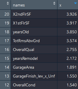
I've sorted the view in descending order by VIF value. I believe we can conclude that there are no apparent problems with multicollinearity.

Finally, we have to see how we're doing out of sample, that is, on our test data. We make the model predictions and examine the results as follows:

> step_pred <- predict(step_lm2, tested)

> caret::postResample(pred = step_pred, obs = test_logy)
    RMSE Rsquared     MAE 
 0.12978  0.89375 0.09492 

> caret::postResample(step_lm2$fitted.values, train_reduced$y)
    RMSE Rsquared     MAE 
 0.12688  0.90072 0.09241 

We see the error increases only slightly: 0.12688 versus 0.12978 in the test data. I think we can do better with our MARS model. Let's not delay in finding out.