
chapter 1
Structural Equation Models
The Basics
Structural tequation modeling (SEvaM) is a statistical methodology that takes a confirmatory (i.e., hypothesis-testing) approach to the analysis of a structural theory bearing on some phenomenon. Typically, this theory represents “causal” processes that generate observations on multiple variables (Bentler, 1988). The term structural equation modeling conveys two important aspects of the procedure: (a) that the causal processes under study are represented by a series of structural (i.e., regression) equations, and (b) that these structural relations can be modeled pictorially to enable a clearer conceptualization of the theory under study. The hypothesized model can then be tested statistically in a simultaneous analysis of the entire system of variables to determine the extent to which it is consistent with the data. If goodness-of-fit is adequate, the model argues for the plausibility of postulated relations among variables; if it is inadequate, the tenability of such relations is rejected.
Several aspects of SEM set it apart from the older generation of multivariate procedures. First, as noted above, it takes a confirmatory, rather than exploratory, approach to the data analysis (although aspects of the latter can be addressed). Furthermore, by demanding that the pattern of intervariable relations be specified a priori, SEM lends itself well to the analysis of data for inferential purposes. By contrast, most other multivariate procedures are essentially descriptive by nature (e.g., exploratory factor analysis), so that hypothesis testing is difficult, if not impossible. Second, whereas traditional multivariate procedures are incapable of either assessing or correcting for measurement error, SEM provides explicit estimates of these error variance parameters. Indeed, alternative methods (e.g., those rooted in regression, or the general linear model) assume that an error or errors in the explanatory (i.e., independent) variables vanish. Thus, applying those methods when there is error in the explanatory variables is tantamount to ignoring error, which may lead, ultimately, to serious inaccuracies—especially when the errors are sizeable. Such mistakes are avoided when corresponding SEM analyses (in general terms) are used. Third, although data analyses using the former methods are based on observed measurements only, those using SEM procedures can incorporate both unobserved (i.e., latent) and observed variables. Finally, there are no widely and easily applied alternative methods for modeling multivariate relations, or for estimating point and/or interval indirect effects; these important features are available using SEM methodology.
Given these highly desirable characteristics, SEM has become a popular methodology for nonexperimental research where methods for testing theories are not well developed and ethical considerations make experimental design unfeasible (Bentler, 1980). Structural equation modeling can be utilized very effectively to address numerous research problems involving nonexperimental research; in this book, I illustrate the most common applications (e.g., in Chapters 3, 4, 6, 7, and 9), as well as some that are less frequently found in the substantive literatures (e.g., in Chapters 5, 8, 10, 11, and 12). Before showing you how to use the Mplus program (Muthén & Muthén, 2007–2010), however, it is essential that I first review key concepts associated with the methodology. We turn now to their brief explanation.
Basic Concepts
Latent Versus Observed Variables
In the behavioral sciences, researchers are often interested in studying theoretical constructs that cannot be observed directly. These abstract phenomena are termed latent variables.1 Examples of latent variables in psychology are depression and motivation; in sociology, professionalism and anomie; in education, verbal ability and teacher expectancy; and in economics, capitalism and social class.
Because latent variables are not observed directly, it follows that they cannot be measured directly. Thus, the researcher must operationally define the latent variable of interest in terms of behavior believed to represent it. As such, the unobserved variable is linked to one that is observable, thereby making its measurement possible. Assessment of the behavior, then, constitutes the direct measurement of an observed variable, albeit the indirect measurement of an unobserved variable (i.e., the underlying construct). It is important to note that the term behavior is used here in the very broadest sense to include scores derived from any measuring instrument. Thus, observation may include, for example, self-report responses to an attitudinal scale, scores on an achievement test, in vivo observation scores representing some physical task or activity, coded responses to interview questions, and the like. These measured scores (i.e., the measurements) are termed observed or manifest variables; within the context of SEM methodology, they serve as indicators of the underlying construct that they are presumed to represent. Given this necessary bridging process between observed variables and unobserved latent variables,it should now be clear why methodologists urge researchers to be circumspect in their selection of assessment measures. Although the choice of psychometrically sound instruments bears importantly on the credibility of all study findings, such selection becomes even more critical when the observed measure is presumed to represent an underlying construct.2
Exogenous Versus Endogenous Latent Variables
It is helpful in working with SEM models to distinguish between latent variables that are exogenous and those that are endogenous. Exogenous latent variables are synonymous with independent variables; they “cause” fluctuations in the values of other latent variables in the model. Changes in the values of exogenous variables are not explained by the model. Rather, they are considered to be influenced by other factors external to the model. Background variables such as gender, age, and socioeconomic status are examples of such external factors. Endogenous latent variables are synonymous with dependent variables and, as such, are influenced by the exogenous variables in the model, either directly or indirectly. Fluctuation in the values of endogenous variables is said to be explained by the model because all latent variables that influence them are included in the model specification.
The Factor Analytic Model
The oldest and best known statistical procedure for investigating relations between sets of observed and latent variables is that of factor analysis. In using this approach to data analyses, the researcher examines the covariation among a set of observed variables in order to gather information on their underlying latent constructs, commonly termed factors within the context of a factor analysis. There are two basic types of factor analyses: exploratory factor analysis (EFA) and confirmatory factor analysis (CFA). We turn now to a brief description of each.
EFA is designed for the situation where links between the observed and latent variables are unknown or uncertain. The analysis thus proceeds in an exploratory mode to determine how, and to what extent, the observed variables are linked to their underlying factors. Typically, the researcher wishes to identify the minimal number of factors that underlie (or account for) covariation among the observed variables. For example, suppose a researcher develops a new instrument designed to measure five facets of physical self-concept (e.g., [self-perceived] Health, Sport Competence, Physical Appearance, Coordination, and Body Strength). Following the formulation of questionnaire items designed to measure these five latent constructs, he or she would then conduct an EFA to determine the extent to which the item measurements (the observed variables) were related to the five latent constructs. In factor analysis, these relations are represented by factor loadings. The researcher would hope that items designed to measure health, for example, exhibited high loadings on that factor, and low or negligible loadings on the other four factors. This factor analytic approach is considered to be exploratory in the sense that the researcher has no prior knowledge that the items do, indeed, measure the intended factors. (For texts dealing with EFA, see Comrey, 1992; Gorsuch, 1983; McDonald, 1985; Mulaik, 2009. For informative articles on EFA, see Byrne, 2005a; Fabrigar, Wegener, MacCallum, & Strahan, 1999; MacCallum, Widaman, Zhang, & Hong, 1999; Preacher & MacCallum, 2003; Wood, Tataryn, & Gorsuch, 1996. For a detailed discussion of EFA, see Brown, 2006.)
In contrast to EFA, CFA is appropriately used when the researcher has some knowledge of the underlying latent variable structure. Based on knowledge of the theory, empirical research, or both, he or she postulates relations between the observed measures and the underlying factors a priori and then tests this hypothesized structure statistically. For example, based on the proposed measuring instrument cited earlier, the researcher would argue for the loading of items designed to measure sport competence self-concept on that specific factor, and not on the health, physical appearance, coordination, or body strength self-concept dimensions. Accordingly, a priori specification of the CFA model would allow all sport competence self-concept items to be free to load on that factor, but restricted to have zero loadings on the remaining factors. The model would then be evaluated by statistical means to determine the adequacy of its goodness-of-fit to the sample data. (For a text devoted to CFA, see Brown, 2006. And for more detailed discussions of CFA, see, e.g., Bollen, 1989; Byrne, 2003, 2005b; Cudeck & MacCallum, 2007; Long, 1983a.)
In summary, then, the factor analytic model (EFA or CFA) focuses solely on how, and to what extent, observed variables are linked to their underlying latent factors. More specifically, it is concerned with the extent to which the observed variables are generated by the underlying latent constructs, and thus the strength of the regression paths from the factors to the observed variables (the factor loadings) is of primary interest. Although interfactor relations are also of interest, any regression structure among them is not considered in the factor analytic model. Because the CFA model focuses solely on the link between factors and their measured variables, within the framework of SEM, it represents what has been termed a measurement model.
The Full Latent Variable Model
In contrast to the factor analytic model, the full latent variable, otherwise referred to in this book as the full SEM model, allows for the specification of regression structure among the latent variables. That is to say, the researcher can hypothesize the impact of one latent construct on another in the modeling of causal direction. This model is termed full (or complete) because it comprises both a measurement model and a structural model: the measurement model depicting the links between the latent variables and their observed measures (i.e., the CFA model), and the structural model depicting the links among the latent variables themselves.
A full SEM model that specifies direction of cause from only one direction is termed a recursive model; one that allows for reciprocal or feedback effects is termed a nonrecursive model. Only applications of recursive models are considered in this volume.
General Purpose and Process of Statistical Modeling
Statistical models provide an efficient and convenient way of describing the latent structure underlying a set of observed variables. Expressed either diagrammatically or mathematically via a set of equations, such models explain how the observed and latent variables are related to one another.
Typically, a researcher postulates a statistical model based on his or her knowledge of the related theory, empirical research in the area of study, or some combination of both. Once the model is specified, the researcher then tests its plausibility based on sample data that comprise all observed variables in the model. The primary task in this model-testing procedure is to determine the goodness-of-fit between the hypothesized model and the sample data. As such, the researcher imposes the structure of the hypothesized model on the sample data, and then tests how well the observed data fit this restricted structure. Because it is highly unlikely that a perfect fit will exist between the observed data and the hypothesized model, there will necessarily be a differential between the two; this differential is termed the residual. The model-fitting process can therefore be summarized as follows:
Data = Model + Residual
where:
data represent score measurements related to the observed variables as derived from persons comprising the sample;
model represents the hypothesized structure linking the observed variables to the latent variables, and, in some models, linking particular latent variables to one another; and
residual represents the discrepancy between the hypothesized model and the observed data.
In summarizing the general strategic framework for testing structural equation models, Jöreskog (1993) distinguished among three scenarios, which he termed strictly confirmatory (SC), alternative models (AM), and model generating (MG). In the SC scenario, the researcher postulates a single model based on theory, collects the appropriate data, and then tests the fit of the hypothesized model to the sample data. From the results of this test, the researcher either rejects or fails to reject the model; no further modifications to the model are made. In the AM case, the researcher proposes several alternative (i.e., competing) models, all of which are grounded in theory. Following analysis of a single set of empirical data, he or she selects one model as most appropriate in representing the sample data. Finally, the MG scenario represents the case where the researcher, having postulated and rejected a theoretically derived model on the basis of its poor fit to the sample data, proceeds in an exploratory (rather than confirmatory) fashion to modify and reestimate the model. The primary focus, in this instance, is to locate the source of misfit in the model and to determine a model that better describes the sample data. Jöreskog (1993) noted that, although respecification may be either theory or data driven, the ultimate objective is to find a model that is both substantively meaningful and statistically well fitting. He further posited that despite the fact that “a model is tested in each round, the whole approach is model generating, rather than model testing” (Jöreskog, 1993, p. 295).
Of course, even a cursory review of the empirical literature will clearly show the MG situation to be the most common of the three scenarios, and for good reason. Given the many costs associated with the collection of data, it would be a rare researcher indeed who could afford to terminate his or her research on the basis of a rejected hypothesized model! As a consequence, the SC case is not commonly found in practice. Although the AM approach to modeling has also been a relatively uncommon practice, at least two important papers on the topic (e.g., MacCallum, Roznowski, & Necowitz, 1992; MacCallum, Wegener, Uchino, & Fabrigar, 1993) have precipitated more activity with respect to this analytic strategy.
Statistical theory related to these model-fitting processes can be found in (a) texts devoted to the topic of SEM (e.g., Bollen, 1989; Kaplan, 2000; Kline, 2011; Loehlin, 1992; Long, 1983b; Raykov & Marcoulides, 2000; Saris & Stronkhurst, 1984; Schumacker & Lomax, 2004); (b) edited books devoted to the topic (e.g., Bollen & Long, 1993; Cudeck, du Toit, & Sörbom, 2001; Hoyle, 1995a, in press; Marcoulides & Schumacker, 1996); and (c) methodologically oriented journals such as Applied Psychological Measurement, Applied Measurement in Education, British Journal of Mathematical and Statistical Psychology, Journal of Educational and Behavioral Statistics, Multivariate Behavioral Research, Psychological Methods, Psychometrika, Sociological Methodology, Sociological Methods & Research, and Structural Equation Modeling.
The General Structural Equation Model
Symbol Notation
Structural equation models are schematically portrayed using particular configurations of four geometric symbols—a circle (or ellipse; ![]() ), a square (or rectangle;
), a square (or rectangle; ![]() ), a single-headed arrow (
), a single-headed arrow (![]() ), and a double-headed arrow (
), and a double-headed arrow (![]() ). By convention, circles (or ellipses) represent unobserved latent factors, squares (or rectangles) represent observed variables, single-headed arrows represent the impact of one variable on another, and double-headed arrows represent covariances or correlations between pairs of variables. In building a model of a particular structure under study, researchers use these symbols within the framework of four basic configurations, each of which represents an important component in the analytic process. These configurations, each accompanied by a brief description, are as follows:
). By convention, circles (or ellipses) represent unobserved latent factors, squares (or rectangles) represent observed variables, single-headed arrows represent the impact of one variable on another, and double-headed arrows represent covariances or correlations between pairs of variables. In building a model of a particular structure under study, researchers use these symbols within the framework of four basic configurations, each of which represents an important component in the analytic process. These configurations, each accompanied by a brief description, are as follows:
| • | Path coefficient for regression of an observed variable onto an unobserved latent variable (or factor) Path coefficient for regression of one factor onto another factor | |
| • | Path coefficient for regression of an observed variable onto an unobserved latent variable (or factor) Path coefficient for regression of one factor onto another factor | |
| • | Measurement error associated with an observed variable | |
| • | Residual error in the prediction of an unobserved factor |
The Path Diagram
Schematic representations of models are termed path diagrams because they provide a visual portrayal of relations that are assumed to hold among the variables under study. Essentially, as you will see later, a path diagram depicting a particular SEM model is actually the graphical equivalent of its mathematical representation whereby a set of equations relates dependent variables to their explanatory variables. As a means of illustrating how the above four symbol configurations may represent a particular causal process, let me now walk you through the simple model shown in Figure 1.1. To facilitate interpretation related to this initial SEM model, all variables are identified by their actual label, rather than by their parameter label.
In reviewing the model shown in Figure 1.1, we see that there are two unobserved latent factors—social self-concept as it relates to one's peers (SSC PEERS) and peer relations (PEER RELATIONS). These factors (i.e., constructs) are measured by seven observed variables—three considered to measure SSC PEERS (SDQSSCPR, APISSCPR, and SPPCSSCPR) and four to measure PEER RELATIONS (peer activity, peer attachment, peer popularity, and peer network). These seven observed variables function as indicators of their respective underlying latent factors. For purposes of example, let's suppose that (a) the three indicators of SSC PEERS represent subscale scores of social self-concept (i.e., self-perceived relations with peers) as measured by three different measuring instruments (SDQ, API, and SPPC, as previously underlined), and (b) the four indicators of PEER RELATIONS represent total scores based on four different approaches to measuring peer relations (e.g., a sociometric scale, in vivo observations, a self-report, and a teacher rating scale).

Figure 1.1. A general structural equation model.
Associated with each observed variable, and with the factor being predicted (PEER RELATIONS), is a single-headed arrow. However, there is an important distinction between these two sets of single-headed arrows. Error associated with observed variables represents measurement error, which reflects on their adequacy in measuring the related underlying factors (SSC PEERS and PEER RELATIONS). Measurement error derives from two sources: random measurement error (in the psychometric sense) and error uniqueness, a term used to describe error variance arising from some characteristic that is considered to be specific (or unique) to a particular indicator variable. Such error often represents nonrandom (or systematic) measurement error. In contrast, error associated with the prediction of endogenous factors from exogenous factors represents the extent to which this predicted value is in error; it is commonly termed residual error.3 For example, the residual error implied by the related single-headed arrow in Figure 1.1 represents error in the prediction of PEER RELATIONS (the endogenous factor) from SSC PEERS (the exogenous factor).
It is important to note that although both types of errors are termed residuals in Mplus, their distinction is evidenced from their linkage to either a factor or an observed variable. For simplicity, however, I maintain use of the terms error and residual throughout this introductory chapter. Further clarification of these distinctions will emerge as we work our way through the applications presented in Chapters 3 through 12.
It is worth noting that, consistent with the representation of factors in SEM, measurement error and residual error actually represent unobserved variables. Thus, it would seem perfectly reasonable to indicate their presence by means of a small circle. However, I am aware of only one SEM program (AMOS) that actually models error in this way.
In addition to symbols that represent variables, certain others are used in path diagrams to denote hypothesized processes involving the entire system of variables. In particular, one-way arrows leading from one variable to another represent structural regression coefficients and thus indicate the impact of one variable on another. In Figure 1.1, for example, the unidirectional arrow leading from the exogenous factor, SSC PEERS, to the endogenous factor, PEER RELATIONS, implies that peer social self-concept “causes” peer relations.4 Likewise, the three unidirectional arrows leading from SSC PEERS to each of the three observed variables (SDQSSCPR, APISSCPR, and SPPCSSCPR), and those leading from PEER RELATIONS to each of its indicators (peer activity, peer attachment, peer popularity, and peer network), suggest that their score values are each influenced by their respective underlying factors. These path coefficients represent the magnitude of expected change in the observed variables for every change in the related latent variable (or factor). It is important to note that these observed variables typically represent item scores (see, e.g., Chapter 4), item pairs (see, e.g., Chapter 3), subscale scores (see, e.g., Chapter 11), and/or carefully formulated item parcels (see, e.g., Chapter 6).
The one-way arrows leading from the ERROR callouts to each of the observed variables indicate the impact of measurement error (random and unique) on the observed variables. Likewise, the single-headed arrow leading from the RESIDUAL callout to the endogenous factor represents the impact of error in the prediction of PEER RELATIONS.
Structural Equations
As noted in the initial paragraph of this chapter, in addition to lending themselves to pictorial description via a schematic presentation of the causal processes under study, structural equation models can also be represented by a series of regression (i.e., structural) equations. Because (a) regression equations represent the influence of one or more variables on another, and (b) this influence, conventionally in SEM, is symbolized by a single-headed arrow pointing from the variable of influence to the variable of interest, we can think of each equation as summarizing the impact of all relevant variables in the model (observed and unobserved) on one specific variable (observed or unobserved). Thus, one relatively simple approach to formulating these equations is to note each variable that has one or more arrows pointing toward it, and then record the summation of all such influences for each of these dependent variables.
To illustrate this conversion of regression processes into structural equations, let's turn again to Figure 1.1. We can see that there are eight variables with arrows pointing toward them; seven represent observed variables (from SDQSSCPR to SPPCSSCPR on the left, and from peer activity to peer network on the right), and one represents an unobserved latent variable (or factor: PEER RELATIONS). Thus, we know that the regression functions symbolized in the model shown in Figure 1.1 can be summarized in terms of eight separate equation-like representations of linear dependencies as follows:
| PEER RELATIONS | = | SSC PEERS + residual |
| SDQSSCPR | = | SSC PEERS + error |
| APISSCPR | = | SSC PEERS + error |
| SPPCSSCPR | = | SSC PEERS + error |
| peer activity | = | PEER RELATIONS + error |
| peer attachment | = | PEER RELATIONS + error |
| peer popularity | = | PEER RELATIONS + error |
| peer network | = | PEER RELATIONS + error |
Nonvisible Components of a Model
Although, in principle, there is a one-to-one correspondence between the schematic presentation of a model and its translation into a set of structural equations, it is important to note that neither one of these model representations tells the whole story; some parameters critical to the estimation of the model are not explicitly shown and thus may not be obvious to the novice structural equation modeler. For example, in both the path diagram and the equations just shown, there is no indication that the variance of the exogenous latent variable, SSC PEERS, is a parameter in the model; indeed, such parameters are essential to all structural equation models. Although researchers must be mindful of this inadequacy of path diagrams in building model input files related to other SEM programs, Mplus facilitates this specification by automatically incorporating the estimation of variances by default for all independent factors in a model.5
Likewise, it is equally important to draw your attention to the specified nonexistence of certain parameters in a model. For example, in Figure 1.1, we detect no curved arrow between the error associated with the observed variable, peer activity, and the error associated with peer popularity, which suggests the lack of covariance between the error terms. Similarly, there is no hypothesized covariance between SSC PEERS and the residual; absence of this path addresses the common, and most often necessary, assumption that the predictor (or exogenous) variable is in no way associated with any error arising from the prediction of the criterion (or endogenous) variable. In the case of both examples cited here, Mplus, once again, makes it easy for the novice structural equation modeler by automatically assuming these specifications to be nonexistent. These important default assumptions will be addressed in Chapter 2, where I review the basic elements of Mplus input files, as well as throughout remaining chapters in the book.
Basic Composition
The general SEM model can be decomposed into two submodels: a measurement model and a structural model. The measurement model defines relations between the observed and unobserved variables. In other words, it provides the link between scores on a measuring instrument (i.e., the observed indicator variables) and the underlying constructs they are designed to measure (i.e., the unobserved latent variables). The measurement model, then, represents the CFA model described earlier in that it specifies the pattern by which each observed measure loads on a particular factor. In contrast, the structural model defines relations among the unobserved (or latent) variables. Accordingly, it specifies the manner by which particular latent variables directly or indirectly influence (i.e., “cause”) changes in the values of certain other latent variables in the model.
For didactic purposes in clarifying this important aspect of SEM composition, let's now examine Figure 1.2, in which the same model presented in Figure 1.1 has been demarcated into measurement and structural components.
Considered separately, the elements modeled within each rectangle in Figure 1.2 represent two CFA models.6 Enclosure of the two factors within the ellipse represents a full latent variable model and thus would not be of interest in CFA research. The CFA model to the left of the diagram represents a one-factor model (SSC PEERS) measured by three observed variables (from SDQSSCPR to SPPCSSCPR), whereas the CFA model on the right represents a one-factor model (PEER RELATIONS) measured by four observed variables (from peer activity to peer network). In both cases, (a) the regression of the observed variables on each factor and (b) the variances of both the factor and the errors of measurement are of primary interest.
It is perhaps important to note that, although both CFA models described in Figure 1.2 represent first-order factor models, second- and higher order CFA models can also be analyzed using Mplus. Such hierarchical CFA models, however, are less commonly found in the literature. Discussion and application of CFA models in the present book are limited to first- and second-order models only. (For a more comprehensive discussion and explanation of first- and second-order CFA models, see Bollen, 1989; Brown, 2006; Byrne, 2005a; Kerlinger, 1984.)
The Formulation of Covariance and Mean Structures
The core parameters in structural equation models that focus on the analysis of covariance structures are the regression coefficients, and the variances and covariances of the independent variables. When the focus extends to the analysis of mean structures, the means and intercepts also become central parameters in the model. However, given that sample data comprise observed scores only, there needs to be some internal mechanism whereby the data are transposed into parameters of the model. This task is accomplished via a mathematical model representing the entire system of variables. Such representation systems vary with each SEM computer program. In contrast to other SEM programs, Mplus, by default, estimates the observed variable intercepts. However, if the model under study involves no structure on the means (i.e., tests involving the latent factor means are of no interest), these values are automatically fixed to zero. Details related to means and covariance structural models are addressed in Chapter 8.
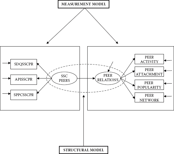
Figure 1.2. A general structural equation model demarcated into measurement and structural components.
The General Mplus Structural Equation Model
Mplus Notation
In general, Mplus regards all variables as falling into one of two categories—measured (observed) variables or unmeasured (unobserved, latent) variables. Measured variables are considered to be either background variables or outcome (i.e., dependent) variables (as determined by the model of interest). Expressed generically, background variables are labeled as x, whereas outcome variables are labeled according to type as follows: Continuous and censored outcome variables are labeled as y, and binary, ordinal (ordered categorical), and nominal (unordered categorical) variables as u. Only continuous and ordinal variables are used in data comprising models discussed in this book.
Likewise, Mplus distinguishes between labels used in the representation of unobserved latent variables, with continuous latent variables being labeled as f and categorical latent variables as c. Finally, unlike most other SEM programs, Mplus models do not explicitly label measurement and residual errors; these parameters are characterized simply by a single-headed arrow. For a comprehensive and intriguing schematic representation of how these various components epitomize the many models capable of being tested using the Mplus program, see Muthén and Muthén (2007–2010).
To ensure a clear understanding of this labeling schema, let's turn to Figure 1.3, a replication of Figure 1.1, recast as an Mplus-specified model within the framework of a generically labeled schema. Given the detailed description of this path diagram presented earlier, no further explanation of the model per se is provided here. However, I would like to present another perspective on the observed variables labeled as y1 through y7. I noted earlier that Mplus labels continuous observed variables as y’s, and this is what we can see in Figure 1.3. However, another way of conceptualizing the labeling of these observed variables is to think of them as dependent variables in the model. Consistent with my earlier explanation regarding the formulation of linear structural equations, each observed variable shown in Figure 1.3 has two arrows pointing toward it, thereby making it a dependent variable (in the model). Possibly due to our earlier training in traditional statistical procedures, we tend automatically, and perhaps subconsciously, to associate the term dependent variable with the label y (as opposed to x). Thus, this generically labeled model may serve to provide you with another way of conceptualizing this full SEM structure.
In this chapter, I have presented you with a few of the basic concepts associated with SEM. Now that you are familiar with these critical underpinnings of this methodology, we can turn our attention to the specification and analysis of models within the framework of Mplus. In Chapter 2, then, I introduce you to the language of Mplus needed in the structuring of input files that result in the correct analyses being conducted. Because a picture is worth a thousand words, I exemplify this input information within the context of three very simple models: a first-order CFA model, a second-order CFA model, and a full SEM model. Further elaboration,together with details related to the analytic process, is addressed as I walk you through particular models in each of the remaining 10 chapters. As you work your way through the applications included in this book, you will become increasingly more confident both in your understanding of SEM and in using the Mplus program. So, let's move on to Chapter 2 and a more comprehensive look at SEM modeling with Mplus.
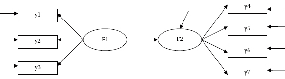
Figure 1.3. A general structural equation model generically labeled within the framework of Mplus.
Notes
| 1. | Within the context of factor analytic modeling, latent variables are commonly termed factors. |
| 2. | Throughout the remainder of the book, the terms latent, unobserved, or unmeasured variable are used synonymously to represent a hypothetical construct or factor; the terms observed, manifest, and measured variable are also used interchangeably. |
| 3. | Residual terms are often referred to as disturbance terms. |
| 4. | In this book, the term cause implies a direct effect of one variable on another within the context of a complete model. Its magnitude and direction are given by the partial regression coefficient. If the complete model contains all relevant influences on a given dependent variable, its causal precursors are correctly specified. In practice, however, models may omit key predictors and may be misspecified, so that it may be inadequate as a “causal model” in the philosophical sense. |
| 5. | More specifically, the Mplus program, by default, estimates all independent continuous factors in the model. |
| 6. | The residual error, of course, would not be a part of the CFA model as it represents predictive error. |