8
PREDICT AND OPTIMISE PLANNING MODELS
Planning is primarily concerned with future performance, and in particular, managing the difference between what could be achieved and what is likely. This requires organisations to understand the impact of business momentum and to challenge whether the current business processes are adequate to reach desired goals.
PREDICTING THE FUTURE
In most surveys on performance, the ability to accurately forecast the future is nearly always at the top of a manager’s wish list. This is because knowing what the future may bring enables them to focus their resources to best effect. For example, if it is known that a product is going to sell 1,000 units a month, then production and raw material purchases can be geared to this level. This in turn reduces working capital requirements by minimising stock levels and eliminates wasted resources that would otherwise go unused. Similarly, if it is known that an investment is not going to deliver the perceived level of return, then a decision can be made earlier to cancel that investment and transfer assigned resources onto projects that are better able to deliver.
However, forecasting is notoriously difficult to do. Not only because of the unknowable and uncontrollable business world that shapes the impact of what we do in the market, but also because the very act of contemplating the future can lead us to do things differently that itself generates a different future from the one we would have obtained.
Believe it or not, organisations do not stop if they do not have a plan or a budget! For most organisations, the momentum of current activities will continue to generate costs and income, irrespective of what is planned. The value of these is fairly easy to forecast in the immediate future but as time goes on, the upper and lower limits of what this could be will diverge, as illustrated in figure 8-1. The reason for the divergence is most likely to be external influences such as competitor actions, market perception about our products, an unexpected change in the cost of raw materials, or a range of other events, most of which are uncontrollable.
Figure 8-1: Impact of Business Momentum and External Events

In recognising this, there are four questions relating to the future that need to be answered:
• What could be achieved by the organisation in the anticipated business environment? That is, what is possible and what is not?
• What is likely to be achieved if things continue as planned? As any person approaching an exam knows, there can be a big difference between ‘what could’ and ‘what is likely’.
• How can the gap between what could be achieved and what is likely to be achiev ed be bridged? In other words, how can resources be optimised within the current plan?
• What fundamental changes are required to make further improv ements? For example, are the current business processes the right ones to deliv er business goals, or should new ones be introduced?
The answer to each question is included in the follow ing logical planning models, which work in conjunction with the operational activity model (OAM) described in chapter 5, ‘Operational Activity Model’:
• Target setting model (TSM). This model answers the question of what could be achieved in the long-term. It takes into account assumed market conditions for the future as well as recent trends in past performance. From this model, senior management can form aspirations about the high-lev el goals that could be achieved, complete with supporting financial statements. Once agreed upon, this is communicated to the rest of the organisation as a top-down plan containing departmental targets.
• Detailed forecast model (DFM). This model looks at the current short-term reality to answer the question of what is likely to happen irrespective of budgets and targets. It takes known facts about revenues and expenses within the current business environment, to build a bottom-up view of the immediate future.
• Optimise resources model (ORM). This third model looks at the most efficient way of aligning current resources with forecast outcomes. It takes a short-term view, but recognises that results should lead to long-term goals. Because of this, any reallocation of resources and effort is bound to be a compromise.
• Strategy improvement model (SIM). This final model allows managers to answer the last question: what can be done about improv ing future performance? This model references the short-term reality, as prov ided by the DFM, and the long-term goals, as set by the TSM. Managers can then assess a range of changes to its business processes that could be implemented either singly or in combination.
The first three models—TSM, DFM, and ORM—are the subjects of this chapter, and the SIM will be covered in chapter 9, ‘Strategy Improvement Model’.
TARGET SETTING MODEL (TSM)
Driver-Based Modelling
The TSM is a simple, idealistic mathematical model that relates the outcomes of organisational business processes (for example, products made, new customers acquired, and customers supported) to long-term objectives and resources. In many ways, it is similar to the OAM, except for the rules that it uses and the versions being held. Whereas the rules within the OAM are used to report the relationships between workload and outcomes, the TSM uses them to generate targets from a range of base data. This is also known as driver-based modelling. In effect, there are a few independent variables, such as forecasted unit sales volume, and the others are dependent variables (for example, based on unit lev el consumption rates and prices).
To illustrate how this works, let’s consider the simple example shown in figure 8-2. In the model, we want to generate a net profit figure by relating the activ ities that contribute to its value. As we did in the example in chapter 5, we ask what driv es net profit, which in our case is rev enue and costs. These are related by the calculation of rev enue less costs.
We now ask what drives each of these elements. If we follow the revenue side of the equation, revenue is calculated from units sold multiplied by price per unit. In our example, management sets the price per unit, and as it is not driven by any thing else, it is called a driver.
Figure 8-2: Simple Example of a Driver-Based Model

We now ask what drives units sold. In the example, this is calculated from the number of orders multiplied by average order size, which is set by management based on past experience, and so becomes a driver. Finally, the example calculates number of orders by multiply ing the number of visits by the sales conversion rate, both of which are entered and are therefore driv ers.
We can now do the same exercise for costs, which we will not do here, but hopefully it is obv ious from figure 8-2. When this analy sis is complete, the relationships identified can be us ed to build a driver-based model where management can enter values into the drivers (for example, number. of visits, conversion rate, average order size, price per unit, and so on), which then uses formulae to create a summary of profit and loss (P&L).
The example covered here is a simple one. More sophisticated models recognise constraints, such as production volumes, the impact of discounts, late delivery penalties, or that more staff will be needed at certain levels of sales. They also recognise that there is nearly always a time lag between the driver and the result it creates. It should also be noted that these models only work for those measures that can be directly related to drivers, such as costs and revenues. Other data, such as overheads, will still need to be included to produce a full P&L summary. Activity-based costing methods address modelling for indirect and shared expenses using similar driver-based principles.
Because of their simplistic nature, driver-based models are not able to take into account unpredictable external influences, such as the unexpected market growth and changes in government legislation that impact taxes. This is where versions come into play. To see the impact of uncontrollable influences, the TSM is set up to hold a variety of scenarios where management can re-run the calculations with different driver values that simulate changing assumptions. For example, the model can be run with different sales conversion rates or unit costs, each of which will generate a new version of the P&L summary. These can then be displayed side-by-side so management can see the impact of each change. A benefit to this model is sensitivity analysis to identify which drivers most impact outcomes.
The aim in doing this is to allow a range of options to be evaluated concerning the future. These options will revolve around business drivers, which, if based on business process outcomes, will cause management to rethink how these are conducted and what could be improved. The end result of the TSM is a scenario that management believes will give them the best outcomes for the available resources. These values are then used to set top-down targets within the OAM that can be referenced by individual departments during the budget process.
TSM Content for XYZ, Inc.
The starting point in deciding the content for the TSM is the output to be fed into target version of the OAM. For our case study, this consists of a high-level P&L statement and the business process outcomes by department. In our example, the TSM does not go down to an activity level, as senior executives want managers at all levels to rethink what these should be once the high-level goals have been set.
From a business dimension point of view, the TSM consists of the following:
• Major product categories.
• Organisational departments.
• Versions including current year actual and current forecast. This dimension is also used to portray a variety of scenarios on predicted performance.
• Time periods that are defined as annual totals, although there is no reason why this could not be at a lower level, such as quarter or month.
• The P&L measures and business goals that are set up as they exist within the OAM. There are also a number of new measures that represent drivers of future performance.
In general, drivers can be grouped into the following types:
• Assumptions. These drivers are those that relate to general changes within the business environment (for example, inflation or market growth).
• Outcome factors. These relate activity to outcomes of a business process (for example, sales conversion rate).
• Industry drivers. These convey an industry specific best practice (for example, stock turn for consumer goods manufacturers).
These drivers are used by rules assigned to the P&L and business process outcome measures. In our case study, they act on past performance to produce future targets, as we will see in the following examples.
In the TSM case study, the drivers used are shown in table 8-1.
Table 8-1: Sample Drivers for the XYZ, Inc. Case Study

The first set is marked as products and contain assumptions about the growth of the market, the expected price, and some basic costs to produce each unit. The first two columns show what is currently being achieved and the latest forecast. These values came from the OAM and cannot be changed. The remaining columns, Year 1-Year 5, are used to enter driver values for the next five years. In our case study, XYZ has five product categories, so this block is repeated for each one.
The second set of drivers, operational costs, relate to various business processes. To keep the example simple, some are assumptions about inflation in different expense categories, and others are industry-specific in that they define the amount a department can spend as a percent of total costs. As with product drivers, the value currently being achieved is displayed alongside the latest forecast to help management set levels for the next five years. These drivers operate on costs at a departmental level.
The last set of drivers also includes assumptions about future tax rates, share ownership, and market size. These are required for calculating the value of key objectives.
The model itself is quite detailed in that it uses the preceding drivers at a product and departmental level. Table 8-2 shows a portion of the model that calculates future revenue targets.
Table 8-2: XYZ, Inc. Case Study Revenue Forecast Generated From Product Drivers

In table 8-2, we have provided a column that explains the driver being used to generate each line. The model accesses data in a prior period and uplifts it according to the value assigned to the driver. For Year 1, the prior year is the current year actual result, which is used to produce the Year 1 target. Year 2 then uses the Year 1 figures and associated drivers to create Year 2, and so on. These calculations are done for revenue and costs at a product level. Subtotal rules then produce summaries that can be used within the P&L statement.
For other costs, the TSM works at a departmental level to produce consolidated costs, as shown in table 8-3.
Table 8-3: XYZ, Inc. Case Study General Costs Forecast Generated From Drivers

It should be emphasised that all of the figures shown in the P&L summary are being driven from the few numbers entered as drivers. Having worked out the details, the TSM then goes on to summarise the business goals and process outcomes that this set of drivers would generate. These are shown in table 8-4.
Table 8-4: XYZ, Inc. Case Study Objectives and Business Process Goals Generated From Drivers

In use, the TSM would hold different versions of the drivers, with each version simulating a particular business scenario. However, each scenario would access the same P&L data. Reports can then be produced that contrasts each scenario so management can see the impact of value driver changes.
As mentioned earlier, the aim of the TSM is to put together a series of targets that could be achieved, provided the assumptions prove correct and the relationships work out as planned.
Using the TSM
The TSM is mainly used during the strategic planning process. This is where senior executives want to review the future direction of the organisation and to challenge management on how they can improve performance.
The forecast and actual version of data held within the TSM are populated from the OAM. This data is stored here for reference purposes and where rules make use of that data to create targets. Prior to this, management will have reviewed past performance as reported in the OAM and supporting detailed history models (DHMs). They would also have looked at future trends in the market, as shown in the performance measures model (PMM). From this, they are now ready to create various scenarios within the TSM that set targets to be achieved for key business performance measures.
As each scenario is created, it should be documented as to the assumptions made about the future business environment. For example, the market grows at 5 percent, bank interest is 4.3 percent, and so on. Where possible, key assumptions affecting a particular set of drivers should be recorded as a measure that can later be compared with what actually happened. Once a particular scenario has been chosen, its values are passed back into the OAM as the target version. This provides the focus for operational managers during the tactical planning or budget process, where they can review their activities and associated costs and work on how those targets could be achieved.
The TSM will not typically determine the level of workload and outcomes of individual business tasks. This is because, in our example, that level of detail is not held within the model and, in the view of the authors, this is better reserved for tactical planning or the budget process. For these processes, the OAM and SIM are the better models to use. However, users will be able to see the high-level targets as set by the TSM.
At a later date, should the assumptions used on the chosen scenario be incorrect or where the business goals are not being achieved, the TSM can be repopulated with the latest actual and forecast data. The TSM is then used to review previous scenarios and create new ones that may become the revised targets for the OAM.
DETAILED FORECAST MODEL (DFM)
Overview
The DFM is typically used in conjunction with the OAM to collect forecasts. Forecasts within the planning framework are defined as values that junior and middle management believe they will realistically achieve in the short term. This can include a range of measures including workload, outcomes, and resources.
Although the OAM can collect forecasts at a summary level, there are measures that benefit from having this at a detailed level. For example, revenue for a manufacturer can come from a range of customers and products, each of which has their individual profitability profile. As a result, the product mix can have huge implications on total revenue and costs. Therefore, to predict profitability with any degree of accuracy requires detailed knowledge of what is being sold, its volume, and to whom.
Similarly, sales of high value items or those that relate to a project are often dependent on timing. In these cases the sales process may be long and when the business is won, the resultant impact on costs and revenues in a particular time period can be significant. Without knowledge of the detail, it is easy tojump to the conclusion that an over- or underperformance is exceptional rather than expected.
For this reason, collecting information concerning the sales order pipeline and using this to populate the sales forecast not only improves accuracy, but also provides insight should any variances occur.
Because different measures can have a wide range of supporting details, there are likely to be multiple forecast models where each has a focus on a particular measure. In the XYZ case study, DFMs exist for sales revenue and personnel costs. As with the DHMs, not every measure warrants its own forecast model. Ideally, they are created for measures where the underlying mix of detailed transactions can have a large impact on results when compared to plan.
Developing the DFM
As previously mentioned, each DFM will typically be focused on a single measure or a range of closely related measures. For example, the case study DFM on personnel holds basic salary, pension, and taxation information, which is then used to populate a number of staffing measures within the OAM.
DFMs will typically hold just a forecast version of data, as actual results will be held in the performance history model. (Remember, we are using the word model in a logical sense; the actual implementation may combine these into one physical model.)
For some measures, data may exist in another system (for example, many companies use SalesForce.com to collect sales information). If this is so, then the DFM may simply be a place where the latest data is stored that is cleared out and repopulated each period. Alternatively, the DFM may be a system in its own right that is used to hold and track forecasts.
In our case study, a DFM was developed as a table to hold sales forecasts with the following fields:
• Date that the sales detail was entered
• Region responsible for the sale and where any revenue will be credited
• Sales executive involved
• Company being sold to
• Type (for example, whether the sale is to an existing customer or a new prospect)
• Product(s) being sold
• Value of the order
• Date contract is due to be signed and revenues recognised in the P&L summary
• Percent chance of the deal going ahead
• Any notes to describe the current situation
Table 8-5: Sales Detailed Forecast Model for the XYZ, Inc. Case Study

Table 8-5 depicts a DFM from our case study. A DFM was also set up for personnel costs that are the same costs as held for the DHM described in the last chapter.
As with the history models, the DFM’s data can be used to sort, analyse, and summarise forecasts. For example, the data can be used to display all sales due in the next three months ranked by the percent chance of them being signed. This enables management to look in detail at the forecasts to form their own opinion as to what could happen and to take remedial action should they fall short of what is expected.
Linking the DFM to the OAM
DFMs contain the breakdown of values for measures held within the OAM. On a regular basis, these details are summarised and the resulting value placed in the forecast version of the respective measures within the OAM.
As an option, the DFM could apply the percent chance measure to the value of each sales situation to produce a modified forecast value within the OAM, or the OAM could contain two measures—one holding a value that assumes all sales opportunities will materialise as held, and the other using the percent chance. This provides a range of values that could be used to assess future performance.
It is worth storing prior forecast versions so that over time, a picture can be built up on the reliability of forecasts. For example, which sales people are able to forecast with an accuracy of 5 percent three months in advance? Which measures produce the most variability when viewed six months in advance? Knowing how trustworthy a forecast is can help determine which measures need regular supervision and provide a more detailed DFM.
Also, if managers are aware that forecasts are being monitored closely, then they are more likely to pay attention to the values they submit, which in turn are more likely to be trusted.
OPTIMISE RESOURCES MODEL (ORM)
Overview
The last type of model to be covered in this chapter is one used to optimise resources. If forecasts about future performance are trustworthy and they differ from what was planned, it may make sense to reallocate some resources to minimise costs or take advantage of them.
Examples of this type of model are those that try to balance production capacity with expected sales volume and mix. Some of these models can be quite sophisticated, particularly for manufacturers that produce in multiple locations and where machines used in manufacture can be configured to produce multiple products.
In this case, the model takes into account where the demand for products exist, what is held in stock at which locations, and the costs involved in transporting finished goods to customers. The model also recognises that to change a machine from producing one product to producing another takes time, and so production will be lost during the changeover period.
Armed with these factors, optimisation models are able to simulate various scenarios to work out what is the best way to minimise production costs and ensure customers receive their orders in the quickest time. This highlights a typical characteristic of these models in that they deal primarily with trade-offs (that is, it is generally not possible to meet all demands of both supplier and customer).
Different industries have different types of trade-offs. Quite often, there are specialised models that can be purchased from vendors to optimise resources, with production scheduling and logistics modelling being good examples. Whatever solution is employed, there should be a link to the OAM or to the appropriate DFM as these will receive the optimised values for subsequent monitoring.
Case Study Example
In the XYZ case study, we have developed a production ORM that seeks to balance what the factory produces with the latest sales forecast in order to minimise stock levels. This model contains stock levels of both raw materials and finished goods as projected by the current production schedule.
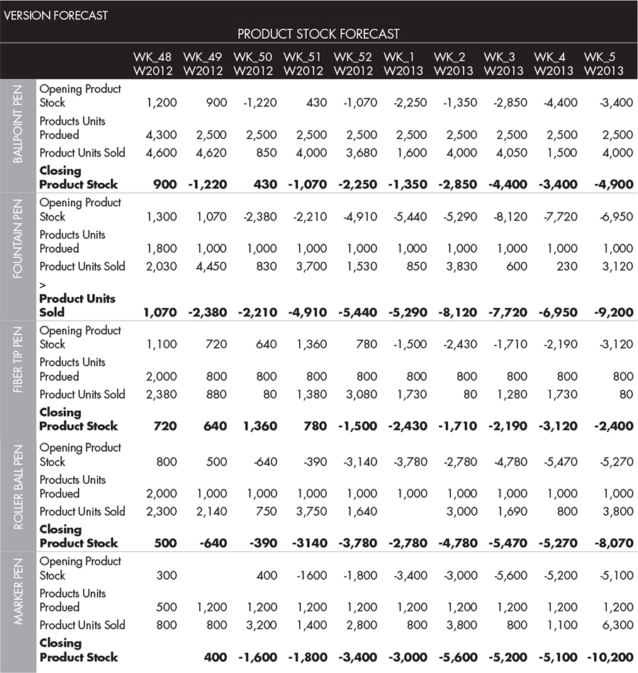
The process starts with each sales division entering a forecast of the units of each product to be sold by customer for the next three months. This is stored in the sales DFM. The production ORM takes this data and compares it to the predicted stock levels of finished products. A report is produced (shown in table 8-6) that shows the status of stock levels by week as adjusted by the sales forecast. Negative values indicate a shortfall in production to meet the forecast.
Table 8-6: Sample Optimise Resources Model Report Showing Where Product Stock Falls Short of the Sales Forecast
Management can now make adjustments to the current production plan to meet the sales forecast. Within the ORM is a recipe that details what raw materials go into which products. As the production volume is adjusted, the ORM is able to compare the stock requirements for raw materials and display this as a report (table 8-7).
Table 8-7: Report Showing Revised Product Stock Levels to Meet Sales Demand

Raw materials can be ordered from suppliers to meet demand.
The result of the ORM is sent back to the OAM as revisions to the resource budget for purchasing goods and manufacturing costs.
The models described so far in this chapter have been used to set targets and to predict and optimise performance in the immediate future. To align the immediate future with the long-range targets will often require a change to the way business is conducted. That is the role of the SIM, which is the subject of the next chapter.