CHAPTER 8

Power System Steady—State Stability Analysis

8.1 Introduction

The stability of a system is broadly defined as the property of the system that enables it to remain in a state of equilibrium under normal operating conditions and to regain an acceptable state of equilibrium after being subjected to a disturbance.

Power system stability is a term applied to a. c. electrical power systems denoting a condition in which the various synchronous machines of a system working in parallel remain in synchronism or in step with each other.

8.2 Forms of Power System Stability

There are three forms of stability conditions that need to be considered for the purpose of analysis, as indicated in Table 8.1.

 

 

Table 8.1 Forms of Stability

8.2.1 Small Signal Analysis

In small signal analysis, the interest is to maintain synchronism among all generating units during or after a small, gradual and slow varying load fluctuation (disturbance) such as those that normally occur in a power system. These small disturbances obviously cannot cause loss of synchronism unless the system is operating at or very near its threshold stability limits, due to the synchronising torque developed by the units. For small variations in load or turbine speed, the system experiences natural oscillations in the machine torque angles, speeds and emfs. The system is said to be stable if the amplitude of these oscillations is small and dies out quickly. The variations in rotor speeds of all synchronous machines cannot be uniform owing to large differences in rotor inertias. Small signal analysis is subdivided into steady-state stability and dynamic stability analysis. The role of automatic voltage regulator (AVR) and speed governor is considered in dynamic stability analysis whereas it is not included in steady-state stability analysis. Dynamic stability is more probable than steady-state stability. Better damping is achieved through the use of power system stabilizers (AVR and Governor). Due to slow variations in the load, these studies are carried out for long durations of up to 30 seconds. Though the power system model is nonlinear, small signal analysis is carried out using the linearized mathematical model. This is because nonlinearities are ignored when the study is carried out for long durations, since a sufficient time for the system can inherently overcome all nonlinearities. The following definitions are important:

1. Stability Limit

It is the maximum power that can be transmitted to the specified location in the power system, under specified operating conditions without loss of synchronism (stability).

Stability limit is the maximum electrical load of the system under the conditions of energy input reaching the threshold value, with the system still operating at equilibrium.

2. Steady-State Stability

Steady-state stability may be defined as the ability of a power system to maintain synchronism between machines within the system and external tie-lines, for small and slow normal load fluctuations.

3. Steady-State Stability Limit

The steady-state stability limit is the maximum power that can be transmitted to the point under concern without loss of synchronism when the disturbance is a slow, sustained and small increase in load.

4. Dynamic Stability

Dynamic stability may be defined as the ability of a power system to remain in synchronism after the initial swing, until the system has settled down to its new steady-state equilibrium condition.

5. Dynamic Stability Limit

If the increase in field current or adjustments in speed settings occur simultaneously with an increase of load from the use of automatic voltage regulators (AVR) and speed governors, the stability limit would be increased significantly. The limit under these conditions is called the dynamic stability limit.

8.2.2 Large Signal Analysis—Transient Stability

In this type of analysis, the system is tested and analyzed for its stability following a large and sudden disturbance. Disturbances such as short circuits, clearing of faults, sudden change in load or loss of lines can be considered in this analysis. Owing to the severity of the disturbance, the analysis is carried for short durations of say up to 1 second. In this short duration, the system cannot overcome nonlinearities: hence nonlinear mathematical models need to be considered for the analysis. The automatic voltage regulators and speed governors are too slow to respond because of their time constants: and are therefore not included in this study.

Transient Stability

Transient stability may be defined as the ability of the system to remain in synchronism during the period following a large and sudden disturbance and prior to the time when governors can act.

Transient Stability Limit

The maximum power which can be transmitted through the system without loss of stability under a sudden and large disturbance is referred to as the transient stability limit.

8.3 Physical Concept of Torque and Torque Angle

This section discusses the basic concepts of torque production in electrical machines, the physical significance of torque angle and its relation with power developed by the machine.

Physical Concept of Torque and Torque Angle

Torque in electrical machines is produced due to the tendency of two magnetic fields to align themselves. In other words, torque is produced due to the interaction of i.e, attraction/repulsion between two magnetic fields.

Consider Figure 8.1. In the figure (a), magnet B is placed in the magnetic field of magnet A such that the opposite poles face each other. The axes of the two magnetic fields are aligned under this condition and the torque produced in the movable magnet B is zero. Hence B cannot move from equilibrium position.

 

 

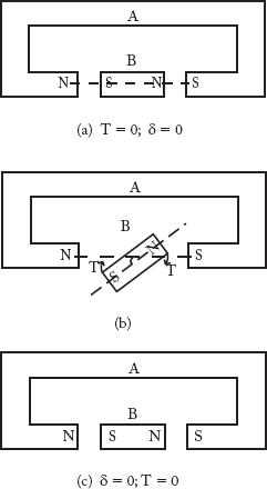
Fig 8.1 Torque Production

 

If a small rotation is given to magnet B as shown in the figure (b) by an angle δ and then released, the force of attraction between opposite poles will give rise to a couple torque T, which will bring back magnet B to its stable equilibrium position as shown in the figure (c). The angle between the axes of the two magnetic fields is called the torque angle (δ).

In the above cases, the torque is not continuous. The free magnet B stops turning when it becomes aligned with the stationary magnetic field axis of A. Figure 8.2 demonstrates how a continuous rotation can be obtained for magnet B. The requirement is that the magnetic field produced by A should be rotating, rather than stationary as in the earlier case.

The figures (a) to (e) demonstrate that if the magnet A is rotated in a particular direction by an angle δ, then the free magnet B will also rotate in the same direction by the same angle.

Let the two magnetic fields be non-aligned by an angle δ as shown in Figure 8.3. The component of force F perpendicular to the axis of the magnet is F₁, which produces the couple torque

 

 

Fig 8.2 Production of Continuous Rotating Torque

 

 

Fig 8.3 Production Couple Torque

 

 

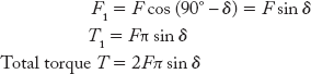
From the above equation it can be concluded that the torque developed is proportional to sin δ, where δ is the torque angle due to non-alignment of two magnetic fields.

8.4 Power Angle Curve and Transfer Reactance

Power angle curve describes the variations in real power for the variations in load, power or torque angle.

Consider a synchronous machine having a direct axis synchronous reactance X_d, which is connected to a large power system such as an infinite bus (where voltage and frequency are maintained constant) through a transmission line having reactance X_t.

The equivalent circuit is shown in Figure 8.4(b).

 

 

Fig 8.4(a) Synchronous Machine Connected to an Infinite Bus

 

Let Voltage behind direct axis synchronous reactance of generator Voltage of infinite bus

Now, the equation for complex power delivered by the generator to the system is:

 

 

 

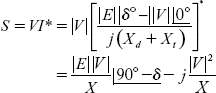
where X = X_d + X_t.

 

 

Fig 8.4(b) Equivalent Circuit for Figure 8.4(a)

 

Separating the real term, the equation for real power delivered to the system is:

 

 

The variation in P_e with δ is shown in Figure (8.5).

 

 

Fig 8.5 Power Angle Curve of Synchronous Generator

 

In the Power angle curve it can be seen that the maximum steady-state power P_m occurs when δ = 90°. The total reactance X which directly connects two emf sources is known as transfer reactance.

Note:

1) The equation for steady-state power limit

2) The steady-state power limit or maximum power limit is inversely proportional to the transfer reactance.

3) Series capacitors can reduce transfer reactance and hence can improve steady-state power limit.

4) For transfer of electrical power, transfer reactance is compulsory. It should not become zero.

5) For transfer of electrical power, resistance is not necessary. However, the condition for P_e to become maximum occurs when

 

 

6) At a particular power angle δ, if transfer reactance is reduced the power transferred in the system increases. This shown in Figure 8.6.

 

 

Fig 8.6 Graph Showing Increase in Power Transfer when Transfer Reactance Value is Reduced

Example 8.1

A synchronous generator having direct axis reactance 0.6 p.u, is supplying full load power with a power factor of 0.85 (lag). The generator is connected to an infinite bus. The voltage at the bus is

1. Find the electrical power transferred to the infinite bus.
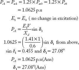
2. If mechanical input is raised by 25% from the previous value, find the new steady-state values of P_e and δ.
3. Now the mechanical input is readjusted to previous value, but excitation is raised by 25%. Find the new steady-state value of δ.

Solution:

1. 
2. 
3. 

Example 8.2

For the system shown in Figure 8.7(a), the per unit reactance values are marked in the figure. Determine the transfer reactance.

 

 

Fig 8.7(a) A Simple Power System

 

 

Fig 8.7(b) Equivalent Circuit

 

Solution:

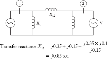
The equivalent circuit of the power system is shown in Figure 8.7(b).

The transfer reactance X between the generator and the infinite bus is given below.

 

Example 8.3

Consider the power system given in Figure 8.8(a). The p. u. reactance values are marked in the figure. Determine the transfer reactance appearing between the generator and the infinite bus.

 

 

Fig 8.8(a) A Single Machine Connected to an Infinite Bus

 

Solution:

The equivalent circuit of the power system in Figure 8.8(a) is given in Figure 8.8(b)

The transfer reactance appearing between the generator and the infinite bus X is given below:

 

 

 

Fig 8.8(b) Equivalent Circuit of Power System Shown in Figure 8.8(a)

Example 8.4

A 3-phase fault occurs at the middle point F on the transmission line as shown in Figure 8.8(a). Determine the transfer reactance appearing between the generator and the infinite bus.

Solution:

The equivalent circuit for the case of fault at point F on line-2 is shown in Figure 8.9(a).

 

 

Fig 8.9(a) Equivalent Circuit of Power System Shown in Figure 8.8(a)

 

It is required to determine the reactance that appears between the generator and the infinite bus. Hence the star network consisting of generator reactance 0.2, Line-1 reactance 0.3 and faulted line half-reactance 0.15 p.u. is converted into equivalent delta network as shown in Figure 8.9(b).

 

 

 

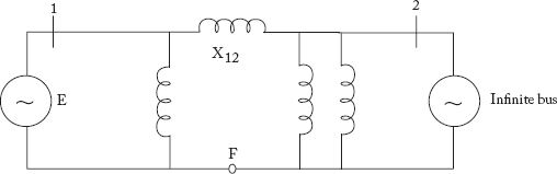
Fig 8.9(b) Transfer Reactance Determination

Example 8.5

Consider the power system shown in Figure 8.7(a). Determine the transfer reactance.

1. if a shunt reactor of 0.15 p.u is connected at midpoint of transmission line
2. if a shunt capacitor of 0.15 p.u is connected at midpoint of transmission line.

Solution:

(a) The equivalent circuit is shown in Figure 8.10(a)

 

 

Fig 8.10(a) A Shunt Reactor Connected to the Middle of the Transmission Line of the Power System Shown in Figure 8.7(a)

 

Two reactances 0.2 and 0.15 p.u are in series. Converting Y-reactance 0.35, 0.15 and 0.15 into delta reactances, the transfer reactance can be determined

 

 

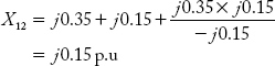
(b) The equivalent circuit is shown in Figure 8.10(b)

 

 

Fig 8.10(b) A Shunt Capacitor Connected to the Middle of the Transmission Line of the Power System Shown in Figure 8.8(a)

 

Converting Y-reactances j0.35, –j0.15 and j0.15 into delta reactances, the transfer reactance can be obtained.

 

Example 8.6

Consider the power system network shown in Figure 8.11(a)

 

 

Fig 8.11(a) Power System Network

 

Generator reactance and terminal voltages are given as:

x¹_d = 0.2 p.u and V_t = 1.0 p.u.

Transfer reactance is 0.1 p.u. Infinite bus voltage is 1.0 p.u. Generator is feeding 1.0 p.u power to the infinite bus. Calculate:

1. Generator emf behind the transient reactance
2. Maximum steady-state power limit that can be transferred under the conditions when i) the system is healthy ii) A 3-phase fault occurs at the middle point of one line iii) the line is opened as a consequence of fault.

Solution:

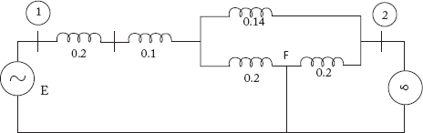
(a) The equivalent circuit of the power system is shown in Figure 8.11(b).

It is given a 1.0. p.u power is transferred from the generator to the infinite bus. From the power angle equation,

 

 

 

Fig 8.11(b) Equivalent Circuit of the Power System Shown in Figure 8.11(a)

 

By substituting numerical values in the equation,

 

 

Voltage behind transient reactance of generator E′ = V_t + IX′_d where generator current I is given as

 

 

(b)(i) System is healthy

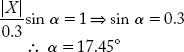
The steady-state power limit P_max is:

 

 

where X₁₂ = transfer reactance = 0.5 p.u

 

 

(ii) The equivalent circuit for this case is shown below.

Converting Y-reactances 0.3, 0.4 and 0.2 into delta reactances, the transfer reactance X₁₂ can be determined.

 

 

 

(iii) When one line is removed, the transfer reactance X₁₂ is the total reactance of the generator, transformer and the remaining line.

 

8.5 The Swing Equation

The swing equation is a second order nonlinear differential equation which describes the rotor dynamics of a synchronous machine. The problem of stability can be understood to be mechanical as well as electrical. When the balance between mechanical input torque (T_m) and electrical power output torque (T_e) is lost, the rotor of an alternator either decelerates or accelerates. The difference between T_m and T_e is the accelerating torque (T_a) and is given by:

 

 

T_a may be positive or negative depending upon the imbalance between T_m and T_e. If T_a is positive, then the rotor accelerates and it retards when T_a is negative. Zero value of T_a indicates that the machine is working at equilibrium.

Note: For the case of a synchronous motor, T_a is the difference of input torque (T_e) and output torque (T_m).

 

 

The speed of the machine may increase or decrease progressively when T_a value is non-zero. The change in speed of different machines cannot be uniform, as accelerating torque depends on mechanical properties of the machine such as kinetic energy and rotor inertia.

From the laws of mechanics, the kinetic energy of a rotating body is given by the following equation:

 

 

Equation (8.3) is analogous to the equation for linear motion of a mass. In Equation (8.3), I is defined as the moment of inertia (analogous to mass) in kilogram-meter² and ω is angular velocity (analogous to linear velocity) in radians/second. Substituting angular momentum (M) = Iω in the Equation (8.3), it can be rewritten as:

 

 

Using the above equation, the unit for M can be derived as Joule-sec per radian. If angular momentum (M) is derived from M = Iω and ω is the synchronous speed of the machine, then M is called the inertia constant. It should be noted that the stored K.E of the rotor depends on the physical structure of the machine such as axial length, diameter of the rotor and gravitational forces acting on the body. The structural design in turn depends on the power output (MVF) of the machine. As there is a relation between stored K.E and the rating of the machine, the inertia constant M is generally computed from another inertia constant H, which is defined as

 

 

From the above equation,

 

 

From Equations (8.3 and 8.6)

 

 

The synchronous speed ω in terms of rated frequency f is:

 

 

By substituting ω in Equation (8.7), the value of M can be computed from the following equations.

 

 

 

Note:

1. The value of M is required to study the stability of the system.
2. In practice, the value of M is computed by using Equation (8.7) rather than by using M = Iω, as H does not vary widely with size. In other words, similar class of machines (say all hydro or thermal) irrespective of their ratings shall have H values in a relatively narrow range. Typical H values for different classes of machine are given below.

   Type of Synchronous Machine	Inertia constant (H) in MJ/MVA
   Turbo generators	3–9
   Waterwheel generators	1.75–4.25
   Synchronous Motors	2.0

3. The value of H is higher for thermal units when compared to that of hydro units.

The Swing Equation

Recalling Equation (8.1) for accelerating torque,

 

 

From the laws of mechanics,

 

 

where I is the moment of inertia in Kg-m² and is the angular acceleration in elec.degree/sec².

 

 

Fig 8.12 Rotor Position with respect to Rotating and Stationary Axes

 

The angular position of rotor (θ) continuously varies with time. It is required to determine the position of the rotor with respect to the synchronously rotating reference axis, rather than with respect to the stationary reference axis as shown in Figure 8.12.

At time t, let

 

 

where ω_s = synchronous speed in elec. degree/sec

δ = Angular displacement of rotor with respect to synchronously rotating reference axis in elec.degrees.

Differentiating Eq. (8.9) on both sides with respect to t,

 

 

and

 

 

Substituting Equation (8.10) in (8.8)

 

 

Multiplying Equation (8.11) with rotor speed ω,

 

 

where M = Iω = Angular momentum P_a, P_m, P_e are accelerating, mechanical input and electrical output powers respectively. Equation (8.12) is known as the swing equation.

From the swing equation,

 

 

where G is the MVA rating of the machines. Taking the rating of the machine as base value, the per unit form of the swing equation is:

 

 

where

 

 

Note:

1. The swing equation describes the rotor dynamics of a synchronous machine (either generator or motor).
2. The swing equation is a second order nonlinear differential equation.

8.6 Modelling Issues in the Stability Analysis

The various components in a power system are modelled as per the discussion presented below to carry out stability studies.

8.6.1 Synchronous Machine Model

The classical model of the synchronous machine is generally used in stability studies. Under transient conditions, the machine is represented as a constant voltage source behind the transient reactance as shown in Figure 8.13.

 

 

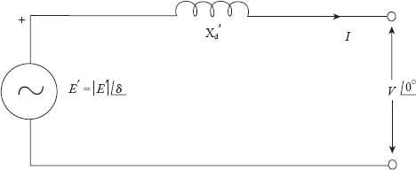
Fig 8.13 Synchronous Machine Model for Stability Studies

Electrical Equations

 

 

In Equation (8.15) the symbols used stand for the usual parameters. The machine model corresponding to Equation (8.15) is valid for both salient and cylindrical rotor machines.

Mechanical Equations

 

 

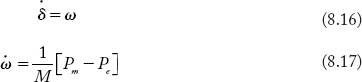
In the Equation (8.17), the damping term due to losses and damper winding is neglected. Eq. (8.17) is from the swing equation.

8.6.2 Power System Model

Power system is divided into two areas, namely, the power exporting area and the power importing area.

 

 

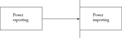
Further, all machines in the exporting area are reduced to an equivalent machine and all machines in the importing area are also converted into another single equivalent one. This reduces the multi-machine system into a two-machine system as shown in Figure 8.14.

 

 

Fig 8.14 A 2-Machine System

 

For simplification, a two-machine system is further reduced to a single machine connected to an infinite bus (SMIB) system as shown in Figure 8.15.

 

 

Fig 8.15 A Single Machine Connected to an Infinite Bus System

Many times, our interest is confined to the study of dynamics of the generator. The simplified SMIB System is widely used by researchers.

8.6.2.1 SMIB System

Figure 8.16 is the circuit model of a single machine connected to the infinite bus through a transmission line of reactance X_e.

 

 

Fig 8.16 SMIB System Trransfer Reactance

For the systme shown in Figure 8.16, the transfer reactance can be obtained as:

 

 

Electrical power transferred

 

 

The dynamics of the SMIB system is described by the swing equation.

 

8.6.2.2 Two-Machine System—Coherent Group

Two machines can form a coherent group i.e., they can accelerate and decelerate simultaneously.

Let the accelerating power of two machines be:

 

 

If these two machines are represented by an equivalent, the stored K.E of the equivalent machine is the sum of the K.Es of the individual machines.

i.e

 

 

where M = M₁ + M₂ or H = H₁ + H₂ is also valid

8.6.2.3 Two-Machine System—Non-Coherent Group

Two machines form a non-coherent group if one machine accelerates while the other decelerates

 

 

Let δ = δ₁ — δ₂, the relative angle between two reference axis, then

 

 

 

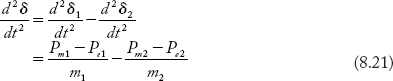
Multiplying both sides of the equation (8.21) by , we have

 

 

Separating the mechanical input and electrical power output terms in the above equation (8.22)

 

 

The above equation (8.23) for the equivalent machine can be written as:

 

 

where, for the equivalent machine,

 

 

or

 

8.6.3 Multi-Machine System

Inertia constant (H) of the equivalent single machine representing a multi-machine system can be obtained as explained below.

Let:

H₁, H₂ …, H_n be the inertia constants of n machines

G₁, G₂ …, G_n be the MVA ratings of n individual machines

The total stored K.E is equal to K.E = H_eG_e = H₁G₁ + H₂G₂ + … + H_nG_n where H_e, G_e are equivalent single machine inertia constant and rating respectively. A single machine stores the total K.E of all the machines.

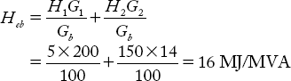
If the inertia constant is to be found on a base G_b, the required equation is:

 

 

 

where H_eb is the per unit inertia constant of the equivalent single machine.

Example 8.7

Two generators rated 200 MVA and 150 MVA are having inertia constants 5 and 4 MJ/MVA respectively. The two machines are put in parallel and are swinging coherently. Therefore find the inertia constant of the equivalent machine on a base of 100 MVA, which represents the two machines

 

Solution:

 

Example 8.8

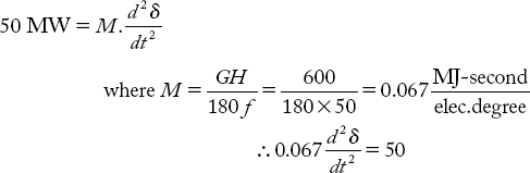
A 50 Hz, 20-pole generator rated 200 MVA, 11 KV has an inertia constant of 3 MJ/MVA. Find

1. the stored kinetic energy in the rotor at synchronous speed.
2. If the prime mover output (generator mechanical input) is raised to 100 MW for an electrical load of 50 MW, find the rotor acceleration in elec.dec/sec²neglecting all losses.
3. If the acceleration of the rotor is maintained for 5 cycles, find the change in torque angle and rotor speed in rpm at the end of the 5-cycle transient period.

 

Solution:

1. Stored K.E = GH = 200 × 3 = 600 MJ
2. Accelerating power P_a = P_m — P_e = 100 — 50 = 50 MW

    

   Therefore,

    

   

    

   or

   

    

3. Time for 5 cycles=5 × = 0.1 sec

    

   

    

   Since the machine is 20-pole machine,

   1 revolution corresponds to 20 × 180 = 3600 elec. degrees

    

   

    

Example 8.9

A power station A consists of two generators G₁ and G₂. The equivalent details are

G₁ = 60 MVA, 50 Hz, 1500 RPM, H₁ = 7 MJ/MVA

G₂ = 100 MVA, 50 Hz, 3000 RPM, H₂ = 4 MJ/MVA

where H is the inertia constant

1. Find the inertia constant of the equivalent generator on a base of 100 MVA.
2. Another power station B has 3 generators whose details are

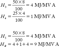
       G₃: 50 MVA, 50 Hz, 1500 RPM, H₃ = 8 MJ/MVA

       G₄: 25MVA, 50 Hz, 1000 RPM, H₄ = 4 MJ/MVA

       G₅: 50MVA, 50 Hz, 3000 RPM, H₅ = 8 MJ/MVA

   Find the inertia constant for the equivalent generator a 100 MVA base.

3. If two power stations are connected through an inter-connector to an infinite bus, replace all the generators with one single machine connected to the infinite bus.

 

Solution:

 

All the units in A form a coherent group (swing together)

(a)On a 100 MVA base,

 

 

The inertia constant of an equivalent single machine representing the power station-A is H_A = H₁ + H₂ = 8.2 MJ/MVA

  (b)All the individual units in B form a coherent group on 100 MVA base

 

 

(c) Two power stations A and B form non-coherent group

 

8.7 Assumptions made in Steady-State Stability Analysis

The following assumptions are made in steady-state stability analysis

1. The study considers small amplitude, long duration perturbations.
2. Nonlinearities are ignored, and hence the linearized form of the swing equation can be used.
3. The damping term in the characteristic equation is absent, because of the assumption of a loss-less system and non-consideration of damper windings
4. The response of the governor and the exciter are ignored. This results in the mechanical power input P_m and the generated emf being considered constant throughout the transient period.

These assumptions lead to pessimistic results at the end of the analysis.

8.8 Steady-State Stability Analysis

This section presents an analysis of the power system for a disturbance of small and slow varying load fluctuations.

Method-1: Using linearized form of the swing equation

Consider a synchronous machine connected to an infinite bus system. The dynamics of the machine is described by the swing equation

 

 

Let the system be operating initially at equilibrium. Neglecting losses, P_eo = P_m1 with torque angle at δ₀. The electrical power output P_e is now slightly increased by ∆P_e, but the mechanical input P_m is fixed.

Due to this, δ increases from δ₀ to δ₀ + ∆δ

As the disturbance is small, we can write the following linearized equation

 

 

Also, from the swing equation,

 

 

or

 

Substituting and in Eq. (8.26)

 

 

The stability of the system for small changes is determined through the characteristic equation

 

 

The two roots of Eq. (8.27) are

 

 

As long as is positive, the two roots are purely imaginary and conjugate to each other. For this condition, the two roots should lie on the j — ω axis, and the motion should be undamped and oscillatory about δ₀. If damping effects such as losses and damper winding presence are considered, these sustained oscillations shall damp quickly.

 

Synchronising power of coefficient

As long as is positive, the system is stable. If < 0, the roots of Eq. (8.28) shall be real with one of them being positive, and the other negative but of equal magnitude. This condition can be easily understood since the torque angle increases without bound upon occurrence of a small disturbance and the synchronism will be lost.

 

 

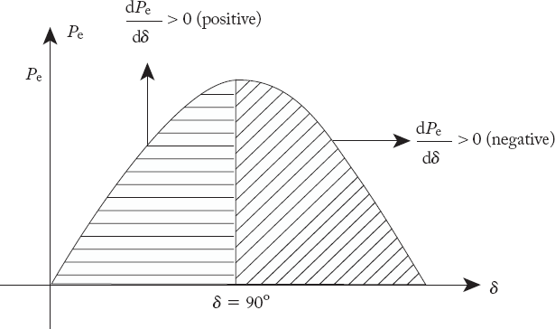
Fig 8.17 Steady State Stability Description Using Synchronizing Power Coefficient

 

The system is therefore unstable for and reaches threshold stability limit for δ = 90˚. At this angle, any further increment in P_e in fact reduces the generated P_c and hence the system loses stability. Though practically not possible, the power system should operate for lower values of δ (say 30 to 40˚) for good stability margins.

The term is known as the “synchronizing power co-efficient”. This is also called stiffness (electrical) of the synchronous machine.

Note:

1) P_r = synchronizing power coefficient =

As discussed earlier, far will be less than zero (negative) and system looses steady state stability.

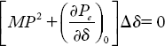
2) Recall the characteristics Eq. (8.26)

 

 

Eq. (8.26) in s-domain can be written as

 

 

or

 

 

Comparing Eq. (8.29) with the standard characteristic equation, the frequency of natural oscillations is given by:

 

 

Equation (8.30) gives the natural frequency of oscillations in δ.

 

Method-2: Eigen value approach

 

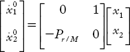
or

 

 

Let the state variables X₁ and X₂ be:

 

 

and

 

 

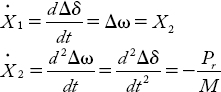
Writing the above equation in the matrix form, we have

 

 

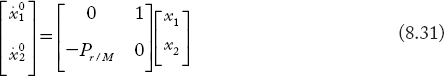
or

 

 

where

 

 

Using the matrix A, the eigen values can be computed. The system shall be stable if all the eigen values are found on the left hand side of s-plane.

Example 8.10

A synchronous generator having a reactance of 1 p.u is connected to an infinite bus through a transmission line. The line reactance is 0.5 p.u. The machine has an inertia constant of 4MW — sec/MVA. Under no load conditions, the generated emf is 1.1 p.u. The system frequency is 50 Hz. Calculate the frequency of natural oscillations, if the generator is loaded to 75% of its maximum power limit.

 

Solution:

 

 

or

 

 

Now,

 

 

Total reactance = x = 1.5 p.u.

 

 

Recalling the formula for ω_n Eq. (8.30)

 

 

Therefore,

 

 

Therefore, the frequency of natural oscillations

 

8.9 Methods to Improve Steady-State Stability

The methods to improve steady-state stability limit include:

Method-1: Reduction of transfer reactance

A power system which has a lower value of transfer reactance can have better steady-state stability limit. This can be achieved by:

1. use of parallel lines
2. use of series capacitors

If the power has to be transferred through long distance transmission lines, use of parallel lines reduce transfer reactance as well as improve voltage regulations. Similarly series capacitors are some times employed in lines to get the same features.

Method-2: Increase in the magnitudes of E and V.

Higher and fast field excitation system enhances steady-state power limits

Questions from Previous Question Papers

1. Define the following terms:

   1. Steady state stability limit
   2. Dynamic state stability limit
   3. Transient state stability limit

2. Give important difference between steady state, transient state and dynamic stability.

3. Define power system stability and stability limit.

4. Define the following terms:

   1. transfer reactance
   2. inertia constant
5. Draw and explain power angle curve of a synchronous machine.
6. Define synchronizing power coefficient and explain its significance.
7. What is steady state stability? Explain it with respect to power angle curve.
8. Discuss the methods to improve steady state stability.

Competitive Examination Questions

1. Steady state stability of a power system is the ability of the power system to

   1. maintain voltage at the rated voltage level
   2. maintain frequency exactly at 50 Hz
   3. maintain a spinning reserve margin at all times

   4. maintain synchronism between machines and on external tie lines.

       

      [GATE 1999 Q.No. 5]

2. A transmission line has a total series reactance of 0.2 p.u. Reactive power compensation is applied at the midpoint of the line and it is controlled such that the midpoint voltage of the transmission line is always maintained at 0.98 p.u. If voltage at both ends of the line are maintained at 1.0 pu, then the steady state power transfer limit of the transmission line is

   1. 9.8 p.u
   2. 4.9 p.u
   3. 19.6 p.u

   4. 5 p.u

       

      [GATE 2002 Q.No. 6]

3. A round rotor generator with internal voltage E₁=2.0 p.u. and X=1.1 p.u. is connected to a round rotor synchronous motor with internal voltage E₂=1.3 p.u. and X=1.2 p.u. The reactance of the line connecting the generator to the motor is 0.5 p.u. When the generator supplies 0.5 p.u. power, the rotor angle difference between the machines will be

   1. 57.42^o
   2. 1^o
   3. 32.58^o

   4. 122.58^o

       

      [GATE 2003 Q.No. 4]

4. An 800 kV transmission line has a maximum power transfer capacity on the operated at 400 kV with the series reactance unchanged, the new maximum power transfer capacity is approximately

   1. P
   2. 2P
   3. P/2

   4. P/4

       

      [GATE 2005 Q.No. 2]

5. A generator with constant 1.0 p.u. terminal voltage supplies power through a step-up transformer of 0.12 p.u. reactance and a double-circuit line to an infinite bus has as shown in figure. The infinite bus voltage is maintained at 1.0 p.u. Neglecting the resistances and susceptances of the system, the steady state stability power limit of the system is 6.25 p.u. If one of the double-circuit is tripped, the resulting steady state stability power limit in p.u. will be

    

   

    

   1. 12.5 p.u
   2. 3.125 p.u
   3. 10.0 p.u

   4. 5.0 p.u

       

      [GATE 2005 Q.No. 10]

6. A 500 MW, 21 kV, 50 Hz, 3-phase, 2-pole synchronous generator having a rated p.f. = 0.9 has a moment of inertia of 27.5 × 10³ kg-m². The inertia constant (H) will be

   1. 2.44s
   2. 2.71s
   3. 4.88s
   4. 5.42s

       

      [GATE 2009 Q.No. 32]