CHAPTER 5

Power Flow Studies—2

5.1 Introduction

This chapter is a continuation of Chapter 4 and discusses power flow solution by the Newton–Raphson (NR), and the decoupled and fast-decoupled methods. Though the Gauss–Seidel method is computationally much easier, it has limitations when applied to large-sized power systems involving more number of unknowns. The methods presented in this chapter are useful for such systems. NR method is very accurate when compared to other methods and guarantees convergence in five to seven iterations irrespective of the size of power system. We compare the NR method with the GS method towards the end of this chapter to appreciate the difference between the two types of power flow solutions. Since the NR method is computationally difficult, the method is simplified with suitable assumptions, leading to the decoupled method and further simplification leading to the fast-decoupled method. Figure 5.1 gives these details.

 

 

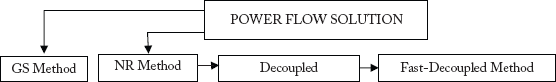
Fig 5.1 Power Flow Solution Methods

 

Before applying the NR method for power flow solutions, it would be helpful to briefly look at the general procedure for solving simultaneous algebraic equations as dealt with in the following section.

5.2 Newton–Raphson Method

The NR method can be applied for linear or non-linear algebraic equations. The method can be easily understood for single-valued functions.

5.2.1 NR Method for Single-Valued Functions

Consider a single-valued function described by

 

 

The solution of Equation (5.1) is the value of ‘x’ at which f (x) = 0.

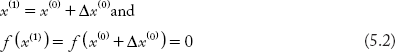
Start with a guess for x as x⁰. Now, we assume the first iteration value of x, x⁽¹⁾ as the solution where,

 

 

The increment ∆x⁽⁰⁾ is not known, but can be estimated by expanding the above equation as a Taylor's series approximation as:

 

 

can be obtained by partial differentiating f(x) with respect to x and then by substituting x = x⁰.

The assumption is that though x⁰ is not the exact solution, it is very close to the real solution. Therefore ∆x⁽⁰⁾ is very small and the higher order terms like ∆²x⁽⁰⁾, ∆³x⁽⁰⁾ … being still smaller, can be neglected. Based on this, Equation (5.3) reduces to:

 

 

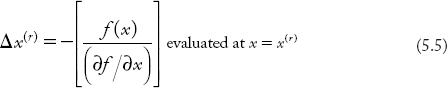
From the above, the value of ∆x⁽⁰⁾ is:

 

 

The first iteration value of x⁽¹⁾ now can be calculated as x⁽¹⁾ = x⁽⁰⁾ + ∆x⁽⁰⁾ and in general the (r + 1)^th iteration value of x is x^{(r + 1)} = x^r + ∆x^r, where:

 

 

and

 

 

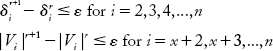
The iteration process shall be terminated when the following convergence condition is satisfied:

, is the error specified

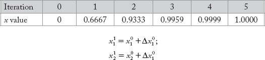
Example 5.1

Find the root of the equation f (x) = x² – 3x + 2 by using Newton–Raphson method

Solution:

Differentiate f(x) with respect to x as:

 

 

Let initial approximation x⁰ = 0

 

 

Using Equation (5.6), the first iteration value of x is,

 

 

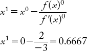
Similarly, consecutive iteration values are

 

 

When x = 1, f(1) = 0 condition is satisfied. Hence the root of the equation is x = 1

5.2.2 NR Method for Multi-Valued Function

Let us apply the NR method for the system of equations where the number of unknowns is more than one. As an example, consider two algebraic equations with two unknown functions x₁ and x₂ as:

 

 

The iteration process is started with guess values for x₁ = x₁⁰ and x₂ = x₂⁰.

The next iteration values of x₁ and x₂ can be obtained by providing error increments to x₁ and x₂ as ∆x₁⁰ and ∆x₂⁰.

 

 

such that Equation (5.7) can be satisfied simultaneously as:

 

 

The error increments can be obtained by expanding Equation (5.8) from Taylor's series approximation as said before and then by neglecting the higher order terms.

Thus,

 

 

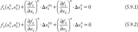
where denotes the partial derivatives of evaluated at x₁ = x₁⁰ while keeping x₂ as constant. Similarly other terms in the Equation (5.9) can be evaluated. The matrix form of Equation (5.9) appears as shown below:

 

 

The condensed form of above equation can be written as

 

 

In Equation (5.10), [J] matrix contains partial derivative terms and it is known as the Jacobian matrix and [∆X] matrix is an increment matrix which is required. In the Equation (5.10) all the matrices except the increment matrix are unknown and can be obtained as:

 

 

The increments can be used to update the x₁ and x₂ values.

 

 

Continue the iteration process till the (r + 1)^th iteration:

 

 

where,

 

 

and terminate, when the following convergence conditions are satisfied simultaneously.

 

 

Equation (5.13) can be generalized for n-unknown variables of n-simultaneous algebraic equations as:

 

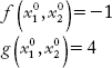
Example 5.2

Use the Newton–Raphson method to solve

 

 

Assume x₁⁰ = 2 and x₂⁰ = –1.

Update the values of x₁ and x₂, perform one iteration

Solution:

Consider Equation (5.9.3). The Jacobian matrix elements are:

 

 

The coefficient matrix elements are:

 

 

The Jacobian Matrix [J] is

 

 

and its inverse is:

 

 

The coefficient matrix is:

 

 

Now, the increment matrix can be obtained as follows:

 

 

The updated values of x₁ and x₂ are:

 

5.3 Power Flow Solution by Newton–Raphson Method

The general procedure for solving simultaneous algebraic equations by Newton–Raphson method is described in Section 5.2. Now, we shall apply the same to power flow problems. NR method can be applied to the power flow problem in two ways, depending upon how bus voltages are expressed. Bus voltages may be expressed in the polar form or in the rectangular form.

5.3.1 NR Method when Bus Voltages are Expressed in the Polar Form

Recall the static power flow equations that were derived in Chapter 4.

 

 

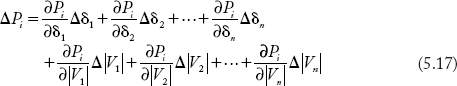
It can be observed in the above equations that the injected P_i and Q_i at each bus in an n-bus power system are functions of n bus voltage magnitudes |V| and another n number of phase angles (δ), totaling 2n bus quantities.

 

 

Since both P_i and Q_i are the functions of 2n quantities, if any one or more quantities changes, the value of both P_i and Q_i changes. The change in |V| and δ can be written with the help of Taylor's series as:

 

 

and

 

 

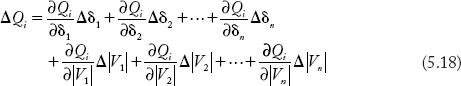
for i = 1, 2,…, n.

We start the NR method for the Case-1 study where PV buses are not present. Bus-1 is slack bus and the rest i = 2,…, n are PQ buses.

The following discussion modifies Equations (5.17) and (5.18).

1. In an n-bus power system, Bus-1 is generally designated as slack bus. For the slack bus, |V₁| and δ₁ are specified. As the specified quantities do not change, the increments (error) ∆|V₁| and ∆δ₁ are zeroes.
2. ∆P and ∆Q denoted are power mismatches, and they represent the difference between specified powers and calculated powers. These are non-zero values owing to an error in |V| and δ values. In the case of PQ buses, specified powers in addition to calculated powers are available and power mismatches can be determined. However, for the slack bus these cannot be determined as the specified powers are not available.

In view of the above, Equations (5.17) and (5.18) can be modified to:

 

 

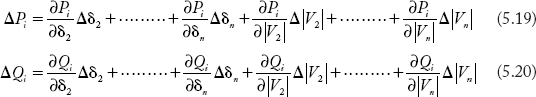
for i = 2, 3,…,n

The above equations can be written as:

 

 

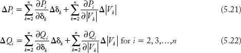
In Equations (5.21) and (5.22), ∆|V_k| is replaced by for the sake of convenience.

 

 

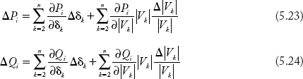
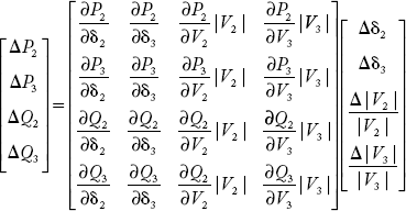
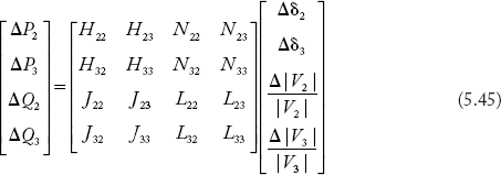
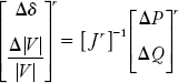
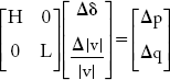
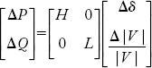
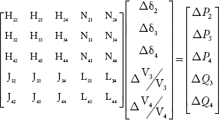
For an n-bus power system, Equations (5.23) and (5.24) can be written in the matrix form as:

 

 

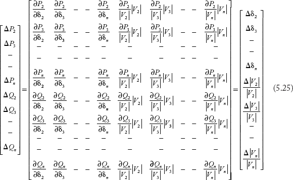
The condensed form of Equation (5.25) is:

 

 

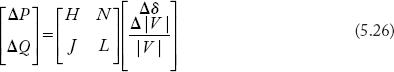
In Equation (5.26), the Jacobian matrix is shown partitioned with sub-matrices H, N, J and L. Any general i^th row and k^th column element of these sub-matrices are:

 

 

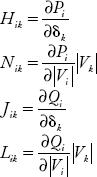
Derivation of Jacobian elements

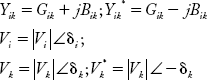
In this section the Jacobian elements are derived while the bus voltages are expressed in polar form. Recall the equation for complex power injected into the i^th bus:

 

 

In the above equation, let

 

 

Substituting above quantities in Equation (4.13):

 

 

Expressing the above equation in rectangular form:

 

 

Separating the real and imaginary terms in the above equation gives:

 

 

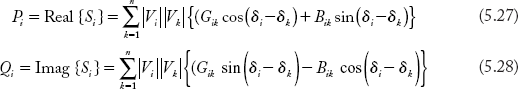
By separating the i^th term in Equation (5.27) and (5.28), they can be written as:

 

 

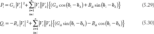
Equations (5.29) and (5.30) can be used to derive the Jacobian elements.

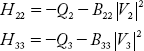
Diagonal elements of H-matrix

 

 

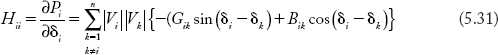
Adding Equations (5.31) and (5.30),

 

 

From the above,

 

 

Off-diagonal elements of H-matrix

 

 

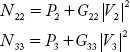
Diagonal terms of N-matrix

 

 

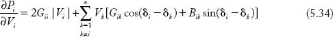
Multiply both sides of Equation (5.34) by |V_i|

 

 

Subtracting Equation (5.29) from (5.34)

 

 

From the above

 

 

Off-diagonal term of N-matrix

 

 

Diagonal term of J-matrix

 

 

Subtracting Equation (5.38) from (5.29),

 

 

Off-diagonal terms of J-matrix

 

 

Diagonal term of L-matrix

 

 

Multiplying Equation (5.41) by |V_i|

 

 

Subtracting Equation (5.30) from (5.42) yields

 

 

From the above,

 

 

Off-diagonal term of L-matrix

 

 

Multiplying above equation by |V_k|

 

 

The following example demonstrates the development of Jacobian elements.

Example 5.3

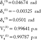
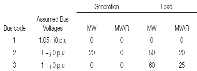
Figure 5.2 represents a 3-bus power system. Develop the network equations for power flow study according to NR Method. Bus 1 is the slack bus and buses 2 and 3 are PQ type.

 

 

Fig 5.2 A 3-Bus Power System Network

 

Solution:

The dimensions of the Jacobian for an n-bus power system with one slack bus and the remaining PQ buses are (2n – 2 × 2n – 2). The set of equations according to NR method is given by:

 

 

and is the expanded form of the above equation is:

 

 

 

The dimensions of the matrices are determined as shown:

• The size of power mismatch matrix is 2n – 2 × 1. For this example its size is 4 × 1.
• The size of Jacobian matrix is 2n – 2 × 2n – 2. For this example its size is 4 × 4.
• The size of increment matrix is 2n – 2 × 1. For this example its size is 4 × 1.

Jacobian elements

Using Equation (5.32) the diagonal elements of the H sub-matrix are:

 

 

Using Equation (5.33) the off-diagonal elements of the H sub-matrix are:

 

 

Using Equation (5.36) the diagonal elements of the N sub-matrix are:

 

 

Using Equation (5.37) the off-diagonal elements of the N sub-matrix are:

 

 

Using Equation (5.39) the diagonal elements of the J sub-matrix are:

 

 

Using Equation (5.40) the off-diagonal elements of J sub-matrix are:

 

 

Using Equation (5.43) the diagonal elements of the L sub-matrix are:

 

 

Using Equation (5.44) the off-diagonal elements of L sub-matrix are:

 

 

Consideration of PV Buses

The set of equations described by Equation (5.26) need to be modified for the case where PV buses are present. Let there be ‘x’ number of PV buses.

1. Since the magnitude of voltage is specified for PV-, generator- and voltage- controlled buses, their increment ∆|V|s do not exist. Hence, in the increment matrix the elements corresponding to PV buses should be eliminated. With this, the dimension of the increment matrix reduces to (2n – 2 – x × 1).
2. In the power mismatch matrix, the reactive power mismatch ∆Q corresponding to PV buses cannot be calculated, as reactive powers for these buses are not specified. Hence the size of the matrix reduces to (2n – 2 – x × 1).
3. Due to modifications in other matrices the size of Jacobian now reduces to (2n – 2 – x × 2n – 2 – x).

Example 5.4 explains all these modifications.

Example 5.4

Consider the 3-bus power system given in Example 5.3. The second bus is the PV bus. Show effect of the PV bus in the power mismatch, Jacobian matrix and increment matrices.

Solution:

1. Since Q₂ is not specified

   ∆Q₂ = Q_{2, specified} – Q_{2, calculated} cannot be determined.

2. Since |V₂| is specified, ∆|V₂| does not exist.

   Now, the matrices are modified considering above effects and are shown as below.

 

 

NOTE: In this case, we need to determine less number of Jacobian elements.

 

Algorithm for Newton–Raphson Method

Let the power system consist of total n-number of buses.

Bus 1 is slack bus.

Buses 2, 3,…, x + 1 are x number of PV buses and the remaining

Buses x + 2, x + 3,…, n are PQ buses.

Algorithm for the NR method is as follows:

Step-1:	Read line data and bus data of the given power system.
Step-2:	Use line data form Ybus.
Step-3:	Use the flat start for guess values for bus voltage magnitudes and phase angles. Set Vi(0) = 1 p. u. for i = x + 2, x + 3…, n and δi = 0 radians for i = 2, 3…, n.
Step-4:	Calculate Pi (for the buses i = 2, 3…, n) by using Equation (4.18) and Qi (for the buses i = x + 2, x + 3…, n) by using Equation (4.19). While calculating these powers, use the most recently updated values of bus voltage magnitudes and phase angles.
Step-5:	Check Qimin ≤ Qi ≤ Qimax for PV buses. If Qi is within the limits Go To Step-6 Else set Qi = Qimin or Qimax as the case and treat this ith bus as PQ bus. Re-designate the bus numbers and return to Step-1.
Step-6:	Calculate power mismatches
	where the superscripts s denotes the specified value, r the current iteration number and c denotes the calculated value. The subscript i denotes the bus number.
Step-7:	Calculate the elements of the Jacobian Matrix.
Step-8:	Calculate the increment matrix as
Step-9:	Update voltage magnitudes and phase angles using the increments as:
Step-10:	Check the convergence
	where, ε is the error specified. If all the convergence conditions are satisfied then go to Step-11, otherwise go to Step-3 and start the next iteration.
Step-11:	Using the specified and converged values of bus voltages and phase angles, calculate the injected powers for the slack bus, and the injected reactive powers for the PV buses.
Step-12:	Perform Stage-2 calculations to determine line flows and losses.
Step -13:	END.

The flow chart for power flow solution using the NR method is given in Figure 5.3

 

 

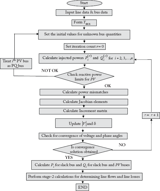
Fig 5.3 Flow Chart for NR Method

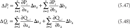
5.3.4 NR Method when Bus Voltages are Expressed in the Rectangular Form

In this method bus voltages are expressed in the rectangular form as:

 

 

The injected P and Q of each bus is a function of all bus voltages and can be written as:

 

 

The power mismatch equations can be written as:

 

 

Equations (5.47) and (5.48) can be represented in the form of a matrix as:

 

 

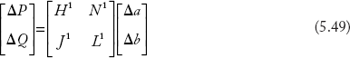
The sub-matrices H¹, N¹, J¹ and L¹ are similar to H, N, J and L as described earlier. Also, the algorithm for this method is similar to the algorithm for Newton–Raphson method, except that the Jacobian elements are evaluated differently. The rectangular version is less reliable as compared to the polar version, though it is slightly faster in convergence. Hence, the rectangular version is rarely used.

Example 5.5

Consider a 3-bus power system shown in Figure 5.4. The line data and bus data are given. The reactive power limits for Bus-2 are Q_{2, min} = 0 and Q_{2, max} = 0.8 p. u.

Update the voltages and phase angles using the NR Method. Perform one iteration. Neglect line changing admittances. All the numerical values are given in p u.

Table: Line Data

Line	Series Impedance
L1	0.025 + j0.1
L2	0.025 + j0.1
L3	0.025 + j0.1

 

 

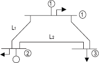
Fig 5.4 A 3-Bus Power System Network

 

Table: Bus Data

 

Solution:

The series admittance of each line is:

 

 

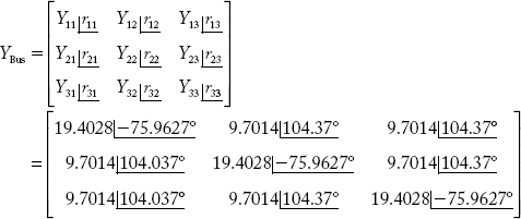
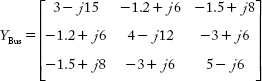
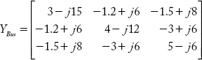
For a 3-bus power system, the size of the Y_Bus is 3 × 3.

The elements of the Y_Bus matrix are:

Y₁₁ = Y₂₂ = Y₃₃ = 4.7059 – j18.8235 p. u.

Y₁₂ = Y₂₁ = Y₂₃ = Y₃₂ = Y₁₃ = Y₃₁ = –2.3529 + j9.418 p. u.

The real and imaginary parts of Y_Bus are given below

G = Real {Y_Bus}

 

 

B = Imaginary {Y_Bus}

 

 

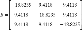
In polar form, Y_Bus is:

 

 

Step-2: Computation of powers

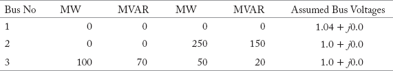
The summary of specified bus quantities is as given below:

Bus-1: V₁ = 1.02 p. u; δ₁ = 0 radians;

Bus-2: P₂ = 1.4 p. u; V₂ = 1.03 p. u;

Bus-3: P₃ = –1.1 p. u; Q₃ = –0.4 p. u;

Assume flat start for bus voltages and phase angles

 

 

The injected active powers can be computed by using Equation. (5.27) as

 

 

The injected reactive powers can be computed by using Equation (5.28)

 

 

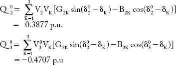
Step-3: Check reactive power limits for PV buses

It may be seen that Q₂⁰ is more than Q_{2, min} and less than Q_{2, max} as:

0 ≤ 0.3877 ≤ 0.8 p. u

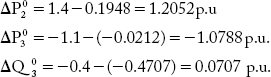
Step-4: Compute power mismatches

Power mismatch is the difference between specified power and computed power.

 

 

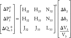
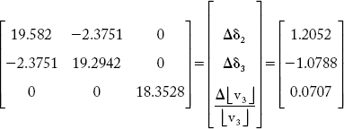
Step-5: Compute Jacobian elements

The power flow matrices for NR method is given below

 

 

H-matrix elements may be computed by using Equations. (5.32) and (5.33)

 

 

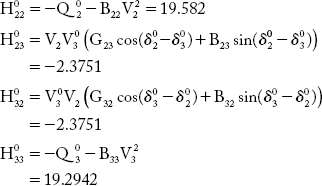
N-matrix elements may be computed by using Equation (5.36) and (5.37)

 

 

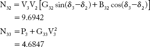
J-matrix elements may be computed by using Equation (5.39) and (5.40)

 

 

The L-matrix elements may be computed by using Equations (5.43) and (5.44)

 

 

Step-6 Compute the increment matrix

 

 

The V-values and modified values of δ are as shown:

 

5.3.5 Comparison of Gauss–Seidel and Newton–Raphson Method

 

5.4 Decoupled Newton Method

The complexities in performing calculations using the NR method are simplified by considering the practical behaviour of the power system. It is understood that P–δ and Q–V are strongly coupled and P–V and Q–δ are weakly coupled. In other words, P is insensitive for variations in V and Q is insensitive for variations in δ. Mathematically,

 

 

Considering the above effect, the set of equations described in Equation (5.26) modifies to:

 

 

Equation (5.50) is the linearised form of Equation (5.26)

 

 

The diagonal and off-diagonal elements of H and L sub-matrices can be obtained by using Equations (5.32, 5.33, 5.43 and 5.44). Equation (5.51a) can be used to find ∆δ. The updated δ values are used in Equation (5.51b) to compute ∆|V|.

5.4.1 Algorithm for Decoupled Power Flow Method

Step-1:	Read line data and bus data of the given power system. Using line data form YBus set iteration count r = 0
Step-2:	Using flat start, assume phase difference δi = 0 radians for PV and PQ buses. |Vi| = 1p.u for PQ buses.
Step-3:	Compute Pi for PV and PQ buses and Qi for PQ buses using the rth iteration voltages and angles.
Step-4:	Check limits Qi,min ≤ Qi ≤ Qi,max for x number of PV buses. If limits are satisfied then go to Step–5, otherwise treat the ith bus as PQ bus go to Step–3.
Step-5:	Compute power mismatches ∆Pi for PV and PQ buses and ∆Qi for PQ buses.
Step-6:	Compute the elements of Jacobian matrix H by using Equations (5.32 and 5.33).
Step-7:	Compute ∆di from ∆Pi = H .∆di for i = 2, 3, 4,…,n
Step-8:	Update angles by
Step-9:	Compute the elements of Jacobian matrix L by using Equation (5.43) and (5.44).
Step-10:
Step-11:	Update the magnitude of bus voltages
Step-12:	Check for convergence
	If all the convergence conditions are satisfied go to Step–13, otherwise increment iteration count and go to Step–3.
Step-13:	Compute slack bus powers and final values of reactive powers for PV buses.
Step-14:	Perform Stage–2 of power flow study to compute line flows and losses.
Step-15:	END.

Example 5.6

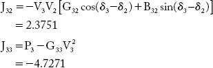
Solve the power flow problem given in Example 5-5 using the decoupled power flow method.

Solution:

The matrices of the NR method are simplified in the decoupled method as:

 

 

Using the numerical results obtained in Example 5-5, the matrices can be written as:

 

 

Substituting the values,

 

 

Solving the above and using the results obtained in Example 5.5, the increments in δ and [v] can be obtained as follows:

 

 

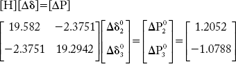
Solving the above,

 

 

and the increments in the voltage are:

 

 

Solving the above,

 

 

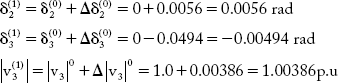
At the end of the first iteration, the updated values of δ and |v|are:

 

5.5 Fast Decoupled Power Flow Method

Decoupled Newton method is a simplified version of the NR method, while fast-decoupled method is a simplified version of the decoupled method. In this method the power flow calculations can be made faster by making suitable assumptions.

Assumption-1: Neglect the angle differences (δ_i – δ_k) such that, cos (δ_i – δ_k) 1 and

 

 

Assumption-2: Power systems generally consist of lengthy transmission network where the ratio X/R is very high. Hence, the resistance of individual elements is neglected against the reactance values. In other words, G_ik can be ignored

 

 

In view of the above assumption, observe the following simplifications:

 

 

In general the value of Q_i is much smaller than

 

 

Considering the above simplifications, the Jacobian elements modify as:

 

 

From the above equations, the following relations can be shown amongst the Jacobian elements:

 

 

Recalling power flow equations of the decoupled method:

 

 

From Equation (5.53), the above matrices can be written as:

 

 

Equation (5.54) can be written as:

 

 

Setting |V_k| = 1 p. u. in Equation (5.55), it can be written as:

 

 

Also, from

The generalized term can be written as:

 

 

Equations (5.56) and (5.57) can be written in the condensed form as:

 

 

In Equations (5.58) and (5.59),

• B′ is the susceptance matrix having the elements – B_ik (for i = 2, 3,…,n and k = 2,3,…,n)
• B″ is part of the susceptance matrix having the elements – B_ik (for i = x + 2, x + 3…, n and k = x + 2, x + 3,…,n) corresponding to PQ buses.

Note: The student is advised to go through numerical problems for better understanding of the extraction of B’ and B” matrices from Y_Bus.

5.5.1 Algorithm for Fast-Decoupled Power Flow Method

The algorithm for power flow solution by the fast-decoupled power flow method is presented below:

Step 1:	Input the line and bus data of the given power system. Set iteration count r = 0.
Step 2:	Form YBus and extract B´ and B″ matrices.
Step 3:	Assume δi0 = 0 radians for i = 2, 3,…,n and
Step 4:	Computer Pi(r) and ∆Pi(r) for i = 2, 3…, n.
Step 5:	Compute δi(r) for i = 2, 3,…,n using Equation (5.58) i.e
Step 6:	Modify and obtain the (r + 1)th iteration value of δi as:
Step 7:	Compute Qi(r) for i = 2, 3,…, n. and ∆Qi(r) for i = x + 2, x + 3,…, n.
Step 8:	Check Qir for limits of PV buses. If satisfied then go to Step-8, otherwise treat the ith bus as PQ bus and go to Step-3.
Step 9:	Compute ∆|Vi| for i = x + 2, x + 3,…, n using Eq. (5.59) i.e.,
Step 10:	Modify |Vi|r+1 for PQ buses using the increment calculated from Step-9.
Step 11:	Check for convergence
	If all the above convergence conditions are satisfied go to Step-12, otherwise increase the iteration count r = r + 1, and go to Step-3.
Step 12:	Compute P1 for slack bus and Q values for slack and PV buses.
Step 13:	Perform Stage-2 calculations. Determine line flows and losses.
Step 14:	END

Some more assumptions made in the FDLF method for further simplifications

Assumption-3:	Omit the elements of B′ that affect the MVAR but not the MW value such as shunt reactance, off-nominal in-phase taps etc.
Assumption-4:	Omit the elements of B” such as the angle shifting effect that predominantly affects MVAR flow. Example: phase shift transformer reactance etc.
Assumption-5:	Neglect the series reactances in calculating the elements of [B].

Power flow solutions can be obtained faster through the assumptions made above. The matrices B′ and B” are real and sparse. These matrices have constant values that need to be evaluated at the beginning of the study.

A flow chart for fast-decoupled power flow method is given in Fig 5.5

Example 5.7

Solve the power flow problem given in Example 5.5 by the fast-decoupled method.

Solution:

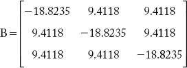
The susceptance matrix B, computed in Example 5.6 is rewritten below:

 

 

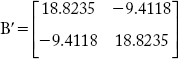
The values for matrices B' and B” in equations (5.58) and (5.59) are extracted from the above B matrix.

B′ matrix corresponding PV and PQ buses (except slack bus)

 

 

Using the results obtained in Example 5.5, increments for ∆δ and ∆|V| can be obtained as follows:

Using Equation (5.58),

 

 

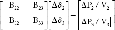
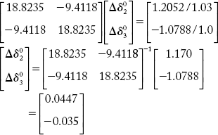
From Equation (5.59),

 

 

From the above,

The updated values of δ and V are:

 

5.5.2 Comparison of NR, Decoupled and Fast Decoupled Power Flow Methods

 

 

 

Fig 5.5 Flow Chart for Fast Decoupled Power Flow Method

 

Example 5.8

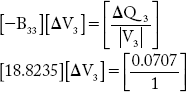
A typical 4-bus power system is shown in Figure 5.6

 

 

Fig 5.6 A 4-Bus Power System Network

 

The line data and bus data are given in the following tables. Neglect charging admittances.

All the values are in p.u.

Table: Line Data

Line No.	Between Buses	Series Impedance of line in P.U.
1	1–2	0.07 + j 0.15
2	1–3	0.06 + j 0.1
3	1–4	0.08 + j 0.25
4	2–4	0.04 + j 0.1
5	3–4	0.04 + j 0.2

Table: Bus Data

 

 

Update the bus voltages and phase angles by performing one iteration and by using

1. NR method
2. Fast decoupled method

Solution:

a) NR method:

Step-1: Obtain Y_Bus by direct inspection method separating the real and imaginary matrices of Y_Bus'

 

 

Step-2: The summary of specified bus quantities are:

V₁ = 1.05 p.u; δ₁ = 0 rad;

P₂ = –0.4; P₃ = –0.5; P₄ = –0.7;

Q₃ = –0.4; Q₄ = –0.2

Step-3: Compute injected powers using Equation (5.27) and (5.28)

P₂^(c) = –0.1767 p.u; P₃^(c) = –0.21955 p.u

P₄^(c) = –0.121155 p.u;

Q₃^(c) = 0.3666 p.u

Q₄^(c) = –0.18082 p.u

Step-4: Calculate power mismatches

∆P₂ = P₂ – P₂^(c) = –0.2233 p.u

∆P₃ = P₃ – P₃^(c) = –0.28045 p.u

∆P₄ = P₄ – P₄^(c) = –0.578845 p.u

∆Q₃ = Q₃ – Q₃^(c) = –0.0334 p.u

∆Q₄ = Q₄ – Q₄^(c) = –0.01918 p.u

Step-5: Compute Jacobian elements

The network matrices for NR Method for the power system shown are given below:

 

 

The procedure for calculating the Jacobian elements can be referred to from the previous examples. The Jacobian matrix is given below.

 

 

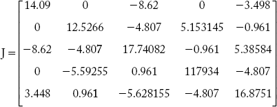
The increment matrix can be obtained by multiplying the [J]⁻¹ with the power mismatch matrix. The increment matrix is given below.

 

 

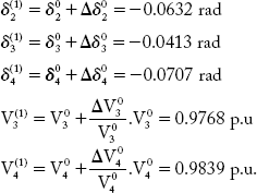
Updated values of δ and V are

 

 

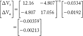
b) Fast-Decoupled Method:

The imaginary component B matrix of the Y_Bus was given earlier. The B' and B” matrices are given below:

 

 

Increments for phase angles can be calculated as:

 

 

Increments for bus voltage magnitudes can be calculated as:

 

 

Substituting the numerical values in the matrices, increments are computed as shown below:

 

 

The updated phase angles and voltages are:

 

 

Questions from Previous Question Papers

1. Derive the power balance equation in a power system and explain the N–R method of load flow analysis. Draw the flow chart giving the sequence of analysis. Show that the polar coordinate representation is advantageous over the rectangular coordinates.
2. Explain the advantages of using the bus admittance matrix in load flow studies.
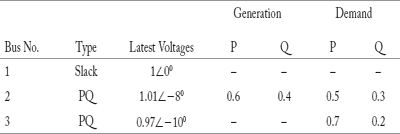
3. Consider the single line diagram of a power system shown in Figure Q1: Take Bus-1 as the slack bus. The Y_Bus matrix is given below

    

   

    

   The scheduled generation and loads are as follows:

    

   

    

   Using the Newton–Raphson method, obtain the bus voltages at the end of the first iteration.

    

   

    

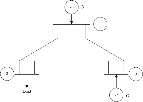
   Fig Q1

    

4. With the data given below, obtain V₃ using N.R method after the first iteration.

    

   

    

   Fig Q2

   Bus code p-q	Impedance Zpqp.u
   1–2	0.08 + j0.24
   1–3	0.02 + j0.06
   2–3	0.06 + j0.18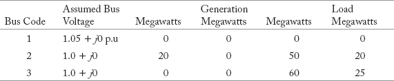

    

   

    

5. Develop from basics, the equations for determining the elements of the H- and L- matrices in the fast decoupled method. State the assumptions that are made for faster convergence.
6. 1. Describe the Newton–Raphson method for the solution of power flow equations in power systems.
   2. What are P–V Buses? How are they handled in the above method?
7. For the network shown in Figure Q3, obtain the complex bus bar voltages at Bus-2 at the end of the first iteration, using the fast-decoupled method. Line impedances are in p. u. Given that Bus-1 is a slack bus with

    

   

    

   

    

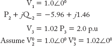
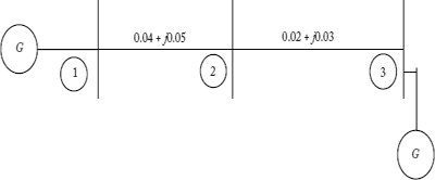
   Fig Q3

    

8. A sample power system is shown in Figure Q7. Determine V₂ and V₃ by the N.R method after one iteration. The p. u. values of line impedances are as shown:

    

   

    

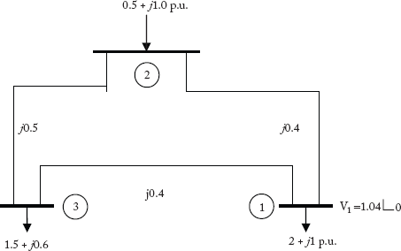
   Fig Q4

    

9. Carry out one iteration of load flow solution for the system shown in Figure Q1, using the fast-decoupled method. Take Q limits of Generator-2 as

    

   

    

10. Find δ₂ and Q₂ for the system shown in Figure Q5. Use the N.R method up to one iteration.

     

    

     

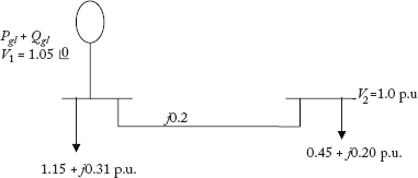
    Fig Q5

     

11. Derive the algorithm for fast decoupled power flow analysis and give the steps for implementation of this algorithm.
12. 1. Obtain the decoupled load flow model starting from the Newton–Raphson method.
    2. What are the assumptions made in fast-decoupled method to speed up the rate of convergence?
13. For the system shown in Figure Q6, find the bus voltage at the receiving end at the end of the first iteration. The load is 2 + j0.8 p.u. Voltage at the sending end (slack) is 1 + j0 p.u. The line admittance is 1.0 – j4.0 p.u. and the transformer reactance is j0.4 p.u. Use the decoupled load flow method. Assume V_r = 10⁰ (Nov-2006)

     

    

     

    Fig Q6

     

14. Consider the given three-bus system. The p.u. line reactances are as indicated in Figure Q7. The line resistances are negligible.

     

    

     

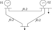
    Fig Q7

     

    The data of bus voltages and powers are given below

     

    

     

    Determine the load flow solution to be solved using the decoupled method for one iteration.

15. Give the general form of load flow equation to be solved in the Newton–Rapshon method. Explain in detail, the approximations in Newton–Raphson method to arrive at decoupled methods.
16. State merits and demerits of the fast-decoupled method.
17. Derive the power balance equations in a power system and explain the N-R method of load flow analysis. Draw the flow chart giving the sequence of analysis. Show that the polar coordinate representation is advantageous over the rectangular coordinates (Or) Describe the Newton–Raphson method for the solution of power flow equations in power systems deriving necessary equations.
18. Explain briefly what do you understand by load flow solution. Obtain the mathematical model for the above study using NR Method. Use the polar coordinate Method.
19. Give a neat flow chart for NR Method of solving load flow equations using rectangular coordinates. Explain clearly the major steps involved in the solution.
    1. When PV buses are not present
    2. When PV buses are present.
20. Using data given below, obtain V₃ using NR Method after first iteration.

     

    

     

    Fig Q8

     

    Line Data:

    Bus Code P – q	Impedance Zpq (p. 4)
    1–2	0.08 + j0.24
    1–3	0.02 + j0.06
    2–3	0.06 + j0.18

    Bus Data:

     

    

     

    Take base MVA as 100

21. A sample power system is shown in Figure Q9. Determine V₂ and V₃ by NR Method after one iteration. The per unit values of line impedances are shown in figure. Bus data is given below.

     

    

     

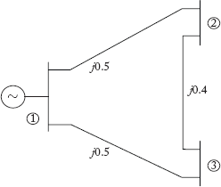
    Fig Q9

     

    Bus Data

    V₁ = 1.04 p.u.; Injected powers S₂ = 0.5 + j1.0 p.u. and S₃ = 1.5 + j 0.6 p.u

22. Consider the single line diagram of a power system shown in Figure Q6. Take bus 1 as slack bus and the Y_Bus is given below

     

    

     

    Scheduled generation and loads are as follows:

     

    

     

    Take base power as 100 MVA.

    Using the NR Method, obtain the bus voltages at the end of 1^st iteration.

     

    

     

    Fig Q10

     

23. Explain the necessary equations for the load flow solution using the NR Method. What is the Jacobian Matrix? Derive necessary equations for computing all the elements of the above matrix using rectangular coordinates.
24. Find |V₂| and S₂ for the system shown in Figure Q11. Use the NR Method upto one iteration.

     

    

     

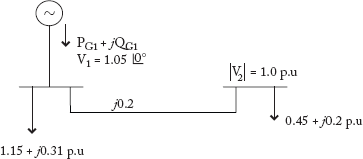
    Fig Q11

     

25. Develop the power flow model using decoupled method and explain the assumptions made to derive at the fast decoupled load flow method. Draw the flow chart and explain.
26. Explain with a flow chart, the computational procedure for load flow solution using fast decoupled method, deriving necessary equations.
27. Develop the equations for determining the elements of H and L matrices in the fast decoupled load flow method, from the basics. State the assumptions that are made for faster convergence.
28. State merits and demerits of fast decoupled load flow method.
29. Compare the GS, NR and FDLF methods.
30. For the system shown in Figure Q12, find the voltage at the receiving end bus at the end of first iteration. Load is 2 + j0.8 p.u. Voltage at the sending end (slack) is (1 + j0) p.u. Line admittance is 1 - j4 p.u. Transformer reactance is j0.4 p.u. Use the decoupled load flow method. Assume V_R = 1 p.u.

     

    

     

    Fig Q12

     

31. For the network shown in Figure Q13, obtain the complex bus bar voltages at bus (2) at the end of first iteration using fast decoupled Method. Line impedances are in p.u. Given bus (1) is slack bus with V₁= 1 ,

     

    

     

    

     

    Fig Q13

     

32. Carry out one iteration of load flow solution for the system shown by fast decoupled method for the network shown in Figure Q14. Take Q limits of generator -- as : Q ₂, min = 0; Q ₂,max = 5

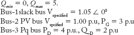
    Bus 1: slack bus V_specified = 1.05 p.u.

    Bus 2: PV bus |V_specified | = 1.00 p.u, P_G2 = 3 p.u.

    Bus 3: PQ bus P_D3 = 4 p.u.; Q_D3 = 2 p.u.

     

    

     

    Fig Q14

     

33. Consider the three bus system shown in Figure Q17. The p.u. line reactances are indicated on the figure. The line resistances are negligible.

     

    

     

    Fig Q15

     

    The data of bus voltages and powers are given below.

     

    

     

    Determine the load flow solution to be solved using the decoupled method for one iteration.

Competitive Examination Questions

1. Load flow studies involve solving simultaneous
   1. linear algebraic equations
   2. non-linear algebraic equations
   3. linear differential equations
   4. non-linear differential equations
2. The principal information obtained from load flow studies in a P.S pertains to the
   1. magnitude and phase angle of the voltage at each bus
   2. reactive and real power flows in each of the lines
   3. total power loss in the network
   4. transient stability limit of the system
   1. 1 and 2
   2. 3 and 4
   3. 1, 2 and 3
   4. 2 and 4
3. A power system consists of 300 buses, out of which 20 are generator buses, 25 are ones with reactive power support and 15 are ones with fixed shunt capacitors. All the other buses are load buses. It is proposed to perform a load flow analysis for the system using N-R method. The size of the Newton-Raphson Jacobian matrix is
   1. 553 × 553
   2. 540 × 540
   3. 555 × 555
   4. 554 × 554

    

   [GATE 2003 Q.NO 12]

4. For a 15-bus power system with a 3-voltage controlled bus, the size of the Jacobian matrix is
   1. 11 × 11
   2. 12 × 12
   3. 24 × 24
   4. 25 × 25

    

   [IES 1996 Q.NO 113]

5. In the solution of a load flow equation, the Newton–Raphson method is superior to the Guass–Siedel method, because the
   1. time taken to perform one iteration in the NR method is less than that in the GS method
   2. number of iterations required in the NR method is more when compared to that in the GS method
   3. number of iterations required is not independent of the size of the system in the NR method
   4. convergence characteristics of the NR method are not affected by the selection of slack bus.

    

   [IES 1997 Q.NO 40]

6. Compared to the Guass–Siedel method, the Newton–Raphson method takes
   1. lesser number of iterations and more time per iteration
   2. lesser number of iterations and less time per iteration
   3. more number of iterations and more time per iteration
   4. more number of iterations and less time per iteration

    

   [IES 1999 Q.NO 49]

7. A 12-bus power system has three voltage-controlled buses. The dimensions of the Jacobian matrix will be
   1. 21 × 21
   2. 21 × 19
   3. 19 × 19
   4. 19 × 21

    

   [IES 2000 Q.NO 67]

8. Match List-I with List-II.

   List-I	List-II
   (Load flow methods)	(System environment)
   A. Guass-Siedel load flow	1. Guass elimination
   B. Newton-Raphson load flow	2. I–V factors
   C. Fast decoupled load flow	3. Contingency studies
   D. Real time load flow	4. Offline solution

    

   [IES 2002 Q.NO 104]

9. Consider the two power system shown in the figure A below, which are initially not interconnected, and are operating in steady state at the same frequency. Separate load flow solutions are computed individually for the two systems, corresponding to this scenario. The bus voltage phasors so obtained are indicated on Figure A. These two isolated systems are now interconnected by a short transmission line as shown in Figure B, and it is found that P₁ = P₂ = Q₁ = Q₂ = 0.

    

   [GATE 2006 Q.No. 11]

    

   

    

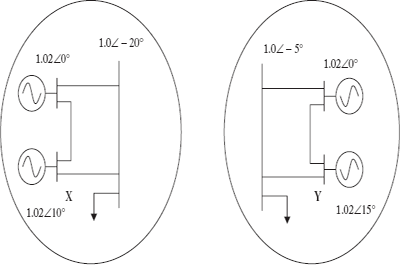
   Figure A

    

   

    

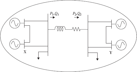
   Figure B

    

   The bus voltage phase angular difference between generator bus X and generator bus Y after the interconnection is:

   1. 10°
   2. 25°
   3. –30°
   4. 30°