CHAPTER 4
Power Flow Studies—1
4.1 Introduction
Satisfactory operation of complex, large and interconnected (grid-operated) power systems requires power flow (commonly called load flow) computer programs. The power flow study program evaluates and analyzes the system under balanced three-phase steady state conditions.
4.1.1 Basic Applications of Power Flow Studies and its Significance in Power System Operation and Control:
- To set the active power generation according to economic-dispatch practice for a given set of active power loads at the bus-bars and transmission loss.
- To set the reactive power generation and transmission in order to maintain the bus voltage magnitudes close to the rated values.
- To verify that generators operate within the specified active and reactive power limits.
- To verify that transmission lines and transformers are not over loaded.
- The study provides the power systems planning engineer with the information necessary to bring about changes in generation and transmission systems to meet projected load growth in the future.
- As the study is conducted under steady-state conditions of the system, it provides numerical steady-state values (initial values at t = 0) of the system parameters for solving differential equations, as in the case of dynamical studies.
- The study is useful for finding the optimal size and location of capacitors to maintain the system's voltage profile at acceptable limits. Likewise, it helps other voltage control equipments like the shunt reactor and static VAR compensators to be installed at proper bus locations.
4.1.2 Data Preparation:
Power flow program is a real time application that runs under on-line condition of the power system. Hence the computers used for this application need high computational speed. A power flow program runs in two stages. Stage-1 results are required to carry out Stage-2. In other words, computation at Stage-1 needs to be completed before the start of Stage–2 calculations.
Stage-1: In this stage four bus quantities are computed at each bus, namely:
- Active power injected into the bus,
- Reactive power injected into the bus,
- Magnitude of the bus voltage, and
- Phase angle (or load/torque angle) of the bus voltage measured with respect to the reference bus voltage.
Power injected (active/reactive) into the bus is the difference between the local power generated and the local power demanded and is the net power available at the bus, which can be transferred to other buses through the transmission lines connected to this bus. If the power generation is more than what is demanded, the injected power is positive and hence, the bus can act as an exporting bus. On the other hand, if the reverse is true, the bus is an importing bus. Also, for an exporting bus the phase angle is leading whereas for importing buses it is lagging. Considering four quantities at each bus for an ‘n’ bus power system, we compute a total of 4n quantities and then go to Stage-2.
Stage 2: This stage can be regarded as the destination stage of the study. In this case, power flows from one bus to another through the transmission line connecting the buses and power loss during the transfer is computed. This computation is performed for each line connecting any two buses.
The Network Model of interconnected power system in the power flow study includes the representation of generators as complex power sources, loads as complex power demands and transmission lines as a Π-network consisting of series admittance and line charging admittances.
The Mathematical Model for the study is a set of nonlinear simultaneous algebraic equations. Network equations in the study can be formulated by using either the ZBus or YBus matrices. However YBus is preferred, as the matrix has more number of zero elements or has more ‘sparsity’. This enables fast solutions using only the non-zero entries.
Either the Gauss–Seidel or the Newton–Raphson iterative method is used to solve non-linear algebraic equations. While the former method is used for small-sized power systems, the latter finds application in the study of large-sized systems. As the study is conducted under steady-state conditions of the system a only a single phase-based positive sequence network is considered and all numerical values are given as per unit values.
4.2 Network Modelling
A practical power system consists of a large number of buses. These buses are interconnected by means of transmission lines. Figure 4.1 represents the single line diagram of a four-bus power system consisting of generators, local demands and transmission lines. In the network model, the power system components are represented as shown in Figure 4.2
- The generator is represented as a complex power source with a complex numerical number. For example, the generator at the ith bus is represented as
SGi = PGi + j QGi
where, SGi, PGi, QGi stand respectively for the complex power, active power, and reactive power generated at the ith bus.
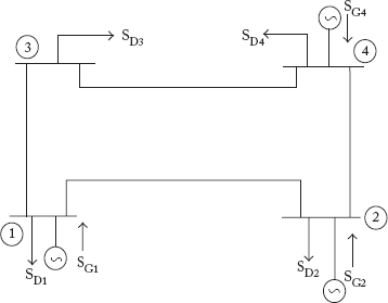
Fig 4.1 Single Line Diagram of a Four-Bus Power System Network

Fig 4.2 Network Model of the Power System Shown in Figure 4.1
- Load is represented as a complex power demand at the bus. That is, by a complex numerical number. For example, load at the ith bus is represented as,
SDi = PDi + j QDi
where, SDi, PDi, QDi stand for the complex power, active power and reactive power demand respectively, at the ith bus.
- A transmission line is modeled as a Π–network, with the series impedance of the line given as series admittance and line charging admittance.
Let Rik, Xik and Cik be the resistance, reactance and capacitance of the line connecting two buses i and k respectively. If the series impedance of the line is Zik = Rik + j Xik then the series admittance of the line is Yik = Gik – jBik, where Gik is the conductance and Bik is the susceptance of the line. These values can be obtained from the expressions ![]() p. u. and
p. u. and ![]() p. u. The half-line charging admittance is given by:
p. u. The half-line charging admittance is given by: ![]() p. u.
p. u.
4.3 Mathematical Modelling
The mathematical model for the power-flow study comprises of a set of nonlinear simultaneous algebraic equations for active and reactive powers. These equations have to be developed for the following quantities:
Stage-1:
- Injected active power
- Injected reactive power
- Magnitude of bus voltage
- Phase angle of the bus voltage measured with respect to the reference bus voltage.
Stage-2:
- Equations for active and reactive power flows
- Transmission line loss
Stage-1 is an iterative process to obtain the bus quantities, whereas Stage-2 is a repeated process for finding line flows and loss in each of the lines present in the power system. The following sub-section deals with the mathematical model for Stage-1 and Stage-2 quantities.
4.3.1 Mathematical Model for Stage-1 Quantities
It has been described in Section 4.1 that injected power is the difference between generated power and demanded power at the bus. Now in this section we develop mathematical expressions for both active and reactive power induced i.e., the complex power injected.

Let Si = Pi + jQi be the complex power injected into any bus (i).
where, Pi = PGi – PDi and Qi = QGi – QDi are the net powers injected into the iih bus Let Ii be defined as injected current into the ith bus.
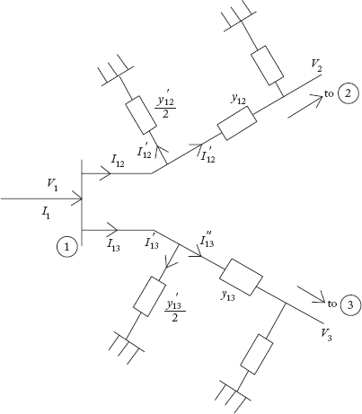
Fig 4.3 Sub–Network of Figure 4.2 for Determining the Injected Current into the First Bus
where,
Considering Figure 4.2 in conjunction with Figure 4.3, the net current injected into the first bus I1 can be written by applying KCL at node 1 as:
Referring to Figure 4.3, the component currents are

Through substitution of the above component currents, the equation for I1is:
y12 and y13 are series admittances while ![]() and
and ![]() are half-line charging admittances of the lines connecting bus (1) to bus (2) and bus (3).
are half-line charging admittances of the lines connecting bus (1) to bus (2) and bus (3).
Rearranging the terms in the Equation (4.3),
Equation (4.4) is written as
where, Y11 = total admittance connected to the first bus ![]()
Y12 = –y12
Y13 = –y13,
Y14 = 0 (since there is no direct connection between buses 1 and 4).
In general, Yii = total admittance connected to the ith bus, and Yik = negative value of series admittance connected between buses (i) and (k); Yik = 0 if the ith bus is not connected to the kth bus.
Following the same procedure as above, the injected currents into the second and third buses can be written as

Putting Equations 4.5–4.8 in the standard matrix form as below:

Since I1, I2, I3, I4 are the currents injected into the buses and V1, V2, V3, V4 are the bus voltages, in the condensed form Equation (4.8) can be written as
For an n-bus power system,
IBus is the n × 1 column matrix representing n-bus currents.
VBus is the n × 1 column matrix representing n-bus voltages.
YBus is the n × n square matrix representing n2 bus admittances.
The elements in the YBus can be computed by direct inspection of the network. This technique of direct inspection and the other methods for YBus formation are presented in Chapter–2. The general expression for the injected current into the ith bus can be written as:
Power flow programs developed by using YBus are more efficient. A comparison of YBus over ZBus, though discussed in Chapter-2, has been repeated here for convenience.
- YBus is a symmetric square matrix, i.e., Yik = Yki.
- YBus is a sparse matrix, i.e. a majority of Yiks are zeros as the each bus may be connected to a maximum of another two to three buses only. As a verification, it can be observed the following terms are zeros in the Eq.(4.9) Y14 = Y41 = Y23 = Y32 = 0.
- It can be observed that the shunt elements such as half-line charging admittances and reactors connected to various buses are present only in the diagonal elements.
- A power flow numerical problem converges quickly if the leading diagonal elements in the YBus dominate over the off–diagonal element. If the reverse happens, the problem diverges.
- The imaginary term representing susceptance is in general negative in the diagonal and positive in the off-diagonal terms of the YBus matrix.
- Chances for convergence of power flow problems increases with the connection of shunt reactors, and decreases with the shunt capacitors at the buses.
- Use of YBus is an example for sparsity techniques. This has following advantages: (1) It reduces computer memory requirements, as only non-zero elements need to be stored. (2) It reduces computation work, thereby improving the speed of power flow application software.
- Now, the equation for the injected complex power Si is arrived at as follows:
The complex power injected into the ith bus is
Substituting Equation (4.10) in (4.12)
Where we use Equation 4.13 for computing Si, it is required to conjugate ‘n’ number of Yik's and Vk's. To reduce the computation time, Si* is calculated instead of Si, where only Vi terms are conjugated as described below:
After solving Equation 4.14 and separating the real and imaginary terms, the equations for injected active and reactive powers can be obtained.
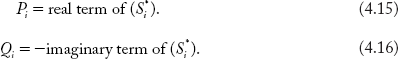
(The minus sign is used because the solution of Equation 4.16 gives a negative value of Qi. To obtain a positive value of Qi, the imaginary term of Si* is negated.)
Let us describe the quantities in equation (4.14) in the polar form as:
where, |V| and δ represent the magnitude of bus voltages and the phase angles respectively and
Substituting the above polar quantities in Equation (4.14), we obtain
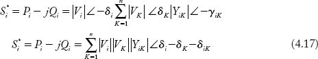
Separating the real and imaginary terms in Equation (4.17),

Equations 4.18 and 4.19 are known as static load flow equations (SLF equations).
Note:
- SLF equations are nonlinear because of the presence of sine and cosine terms.
- The SLF equations can be described as “nonlinear simultaneous algebraic equations.” Now, we develop the equations for the remaining two bus quantities i.e., |Vi| and δi. From Equation (4.14),
or
Separation of K = ith term in the above equation yields,
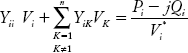
Now, the equation for Vi can be written from the above as:

When Equation 4.20 for Vi is written in the polar form, the values of magnitude and load angle of the ith bus voltage can be obtained. Solving equations (4.18) to (4.20) provides the required four bus quantities.
4.3.2 Mathematical Modeling for Stage-2 Quantities
In this section we discuss the mathematical expressions for computing line flow and loss.
Consider the line connecting buses i and k as shown in Figure 4.4. Let Sik = Pik + jQik be the power transferred from the ith bus to the kth bus, Iik be the current flowing from the ith bus to kth bus, and Vi and Vk be the ith bus and kth bus voltages. Applying KCL at junction (i), Iik can be written as:
Now, the equation for Sik is
Substituting (4.21) in (4.22), the equation for Sik is obtained below
Using Equation 4.23(a), the active and reactive powers transferred from ith bus to the kth bus can be calculated as:
Following the above procedure, the equation for power transferred from the kth bus to the ith bus can be directly written as:
where Pki = active power transferred from the kth bus to the ith bus = real{Sik } and Qik = imag(Sik), the reactive power transferred from the kth bus to the ith bus.

Fig 4.4 Line Flow Calculations
If Pik > Pki the ith bus exports active power, and the kth bus receives it. If on the other hand, Pki > Pik, the kth bus exports active power, and the ith bus receives it.
Now, the summation of Sik and Ski gives the power loss in the transmission line.
The above procedure is repeated for all the l-number of transmission lines and the total loss, as the number of lines, can be obtained.

This concludes the modeling stage of the power flow problem. Power flow equations are nonlinear algebraic equations which cannot be solved directly. These are solved only by application of iterative numerical methods such as the Gauss–Seidel or the Newton–Raphson methods. The power flow solution by Gauss–Seidel method is described in this chapter whereas the Newton–Raphson method of power flow solution is dealt with in Chapter 5.
4.4 Gauss–Seidel Iterative Method
Nonlinear simultaneous algebraic equations can be solved with less computational effort by using the Gauss–Seidel method. As in any iterative method, this method starts with an initial approximate or guess value and progressively in the consequent iterations; more accurate estimates are computed until a final value is reached with the desired accuracy. If the convergence solution is required with a desired accuracy up to the 3rd decimal, then the first three decimal numbers in the final and the previous iteration values should remain the same. In this section we take a closer look at the procedure involved in the Gauss–Seidel method. Let us consider a set of n-nonlinear simultaneous algebraic equations with n number of unknowns.
X1 = f1 (X1, X2,…, Xn)
X2 = f2 (X1, X2,…, Xn)
--------------------------
Xn = fn (X1, X2,…, Xn)
Algorithm:
- Start with initial guess values for x's as: X10, X20,…, Xn
- Estimate the first approximation for X11 as: X1(1) = f1 (X10, X20,…, Xn0)
- Estimate the first approximation for X21 as: X2(1) = f2 (X11, X20,…, Xn0)
- It is to be noted that, in the calculation of X2(1) the already updated value of X1, i.e., X1(1) is used instead of X1(0). In general, Xi1 = fi(X1(1), X2(1),…, Xi – 1(1), Xi(0), Xi +1(0),…, Xn(0)
- The process is continued until ‘r’ number of specified iterations. In general, the rth approximation for Xi is computed as: Xi(r) = Fi (X1(r), X1(r),…, Xi–1(r), Xi(r– 1), Xi+1(r–1),…, Xn(r–1))
- The change in each variable ∆Xi of rth iteration is then examined as ∆Xi(r) = Xir – Xir–1 for i = 1, 2,…, n;
- If ∆Xi(r) for i = 1, 2,…, n <
 (error specified) then the solution is converged.
Use of acceleration factor
The total number of iterations to reach the convergence solution can be reduced by using the acceleration factor. The accelerated Xir value is: Xir = Xir–1 + α (Xir – Xi r–1) where α is a real number called the acceleration factor. The general recommended value of α is 1.6. Example 4.1 describes the general procedure of the Gauss–Seidel Method.
Example 4.1
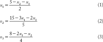
Solve the following equations by using the Gauss–Seidel method.
Solution:
The above equations can be rewritten as:
Assuming the starting values of x2 and x3 as x20 = x30 = 0
Iteration 1: By substituting the current values of x1, x2 and x3 in Equations (1), (2) and (3), the variables are updated as:
Iteration 1:

Iteration 2:

Iteration 3:

+1.808 pt
Iteration 4:

Iteration 5:
Substituting the 4th iteration values of x2 and x3 in Equation (1)

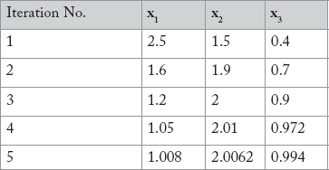
We continue the process until the difference in xi's from current to the previous iteration is very small. The values obtained during the five iterations are given in the following table:
4.5 Classification of Buses
Considering the four bus quantities, at each bus a total of 4n variables need to be found for an n-bus power system in Stage-1. To obtain 4n variables, a total of 4n nonlinear algebraic equations need to be solved in each iteration. As the practical power system consists of a large number of buses, the number of equations and hence iterations also increase proportionately. This has significant impact on executing the power flow problem under online conditions. Hence suitable assumptions such as specification of two out of the four bus quantities shall reduce computational work and computer CPU time. By specifying two variables at each bus, the number of equations reduces to 2n from 4n. This assumption speeds up the process, thereby enabling the study to be carried out under online conditions of the power system.
In an inter-connected power system, the buses are connected with one device or a combination of devices like generators, loads and voltage control equipment. Variables are specified depending upon the equipment connected to the bus. Buses can be classified into 4 types as:
- PQ or load bus.
- PV or generator bus.
- Slack or swing or reference bus.
- Voltage-controlled bus.
4.5.1 PQ Bus or Load Bus
A majority of the buses in a power system are of this type (about 85% of the total buses). At this bus, injected active and reactive powers are specified, and the magnitude and phase angles are unspecified. At each PQ bus, the generated power values PGi and QGi are fixed or specified and the local demanded powers PDi and QDi are known from measurement or by load forecasting. Knowing generation and demand, and the net injected powers at the bus can be calculated as:

The ith bus in the following figure can be designated as the PQ bus

Fig 4.5 Designating ith Bus As Pq Bus, (a) ith Bus Is Either Importing/Exporting, (b) ith Bus Is An Exporting Bus, (c) ith Bus Is An Importing Bus, (d) ith Bus Is An Inter-Connector
In Figure 4.5(a), if PGi > PDi, QGi > QDi, and Pi and Qi are non-zero positive values, then the ith bus can act like an exporting bus. If PGi < PDi and QGi < QDi then the bus acts like an importing bus. Bus i in Figure 4.5(b) is an exporting bus. In Figure 4.5(c) the ith bus is an importing bus while in Figure. 4.5(d), it acts as an inter-connector where, the Pi and Qi values are zeroes.
4.5.2 PV Bus or Generator Bus
A bus can be designated as a PV bus, only when a generator is connected to it. At this bus, the injected active power Pi and the magnitude of the bus voltage |Vi| are specified. About 15% of buses in a power system are of this type.
Justification for specifying Pi and |Vi |
PGi value can be set to a desired value based on the requirements of active power at the importing buses within the permissible control action of the generator. This bus is generally an exporting bus. Within the permissible control action of the exciter, the voltage magnitude can be controlled at this bus. However, as excitation has its limits, the generator at this bus cannot generate reactive power less than QGi,min or more than QGi,max. Knowledge of these reactive power limits is necessary. As long as the Qi value is within the limits, this generator bus can be continued to be treated as the voltage controlled PV bus. However, if in any of the iteration Qi violates the limits, the bus can no longer be treated as a PV bus, and the power flow solution should again be initiated by re-designating this bus as a PQ bus. When it is re-designated, the value of QGi is set to either QGi,min or QGi,max as the case may be.
4.5.3 Voltage Controlled Buses
Because of its capabilities in maintaining bus voltage to the specified value, a PV bus/generator bus may be designated as a voltage controlled bus. However, a pure voltage controlled bus has a basic distinction in that it is connected with only voltage control equipment like SVCs and TCUL transformers, and not generators. Hence at this bus, the following values are known a priori:
PGi = QGi = 0; Pi = – PDi; Qi = – QDi; |Vi| = Specified value and only δi is the unknown parameter.
4.5.4 Slack Bus/Swing Bus/Reference Bus
In a power system, if one bus connected is connected to a generator with high generation capacities (both P and Q), it is designated as the slack bus. At this bus |Vi|and δ are specified, and P and Q are unknown parameters.
Justification for specifying |Vi|and δ:
To find the phase angle difference δ amongst n-bus voltage vectors, one of the voltage vectors is taken as the reference vector. Since slack bus voltage is chosen as the ‘reference vector’, its phase difference δ value is always zero and hence is known to us. As the bus is equipped with a generator, specifying |Vi| is justified.
Justification for un-specifying P and Q
The power balance equations can be written as:
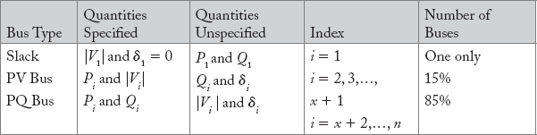
In a power flow study, the generator of active and reactive power cannot be set to the correct values, since the loss in the lines is unknown till the study is complete. Therefore it is necessary to have one bus as the slack bus at which the complex power generation is not initially set. The generation at the slack bus is such that, it supplies the difference in the total system load plus losses minus the sum of the complex powers specified at the remaining buses. In an n-bus power system, for coding convenience bus-1 is always the slack bus, and bus numbers 2, 3, 4,…, x + 1 are assigned to x number of PV buses and x + 2,…, n are assigned to PQ buses.
Summary of classification of buses
4.6 Case Studies in Power Flow Problem
The power flow problem can be discussed in two case studies.
Case 1: The power system consists of the slack bus and PQ buses, but without PV buses
Case-2: The power system consists of the slack bus and PQ buses, with PV buses.
It should be noted that, as the majority of buses are PQ buses, all power flow studies usually include these buses. In addition, without the slack bus, a power flow problem never converges and cannot be solved. However, without PV buses a power flow solution is still possible since some of the PQ buses can act like exporting buses.
4.7 Algorithm for Power Flow Solution by the Gauss–Seidel Method
This Section presents the algorithm for the Gauss–Seidel method for a system with n number of buses.
Step-1: Formation of YBus
Using the line data for resistance, reactance and half-line charging admittance of various lines, form YBus using one of the methods discussed in Chapter-2.
Step-2: Read the bus data for the 2n bus quantities specified.
Before attempting Stage-2 calculations for obtaining the line flows and losses, it is required to find the remaining 2n bus quantities. The Case-1 study is presented in Section 4.7.1 and the Case-2 study in Section 4.7.2.
4.7.1 Case-1: GS Method to obtain Bus Quantities when the PV Buses are Absent
The 2n bus quantities unspecified are: P1, Q1 for the slack bus and |Vi| and δi for i = 2, 3,…, n.
Step-3: Calculation of Bus–Quantities for the PQ buses
Initially assume |Vi| = 1 p.u. and δi = 0 rad for i = 2, 3,…,n (for the PQ Buses). This start is known as Flat-Start. Update these (2n – 2) bus quantities at every step of iteration. Using Equation (4.20), |Vi| and δi can be determined by the GS iterative process as described below:
Now, for the (r + 1)th iteration, the voltage becomes
Updated values of Vkn+1 (k = 1, 2,…, i – 1) are used for this iteration, whereas for the rest of the voltages, the previous values, i.e., Vkr (k = i + 1, i + 2,…, n) are used.
Acceleration for convergence
Convergence in the Gauss–Seidel method can be speeded up by the use of acceleration factor as:
where, α is a real number called the acceleration factor. A suitable value of α for any system can be obtained by the trial process. The recommended value of α for the power flow study is 1.6. A wrong choice of α may slow down convergence or even cause the method to diverge. The iteration process is continued till the convergence solution is obtained when the changes in bus voltages in successive iterations become less than the pre-specified error ε value. After this iteration process has been completed, slack bus powers P1, and Q1 are computed as the last step in Stage-1 power flow calculations.
After obtaining the converged values for all bus voltages, we calculate slack bus powers as shown in Step-4.
4.7.2 Case-2: GS Method to obtain Bus Quantities when the PV Buses are Present
The unspecified bus quantities in this case study are: P1 and Q1 for the slack bus; Qi and δi for i = 2, 3,…, x + 1 of x number of PV buses; and |Vi| and δi for i = x + 2,…, n of PQ buses.
The conditions to be met with PV buses are:
- |Vi| = specified values
- Qi,min < Qi < Qi,max for i = 2, 3,…, x + 1
The second condition shall be violated if the specified voltages are either too low or too high. It is possible to control the |Vi| by Qi. During the iteration process, if Qi violates the prescribed limits, it is fixed to either Qi, min or Qi, max as the case may be and the PV bus should be treated as a PQ bus.
Step-3: Calculation of bus quantities for the PV buses
Active power Pi, for i = 2, 3,…, n is known at the PQ/PV buses, and voltage magnitude |Vi| for i = 2, 3,…, x + 1 is known at the PV buses. Reactive power Qi for i = x + 2,…, n is known at the PQ buses and voltage angle δi for i = 2, 3,…, n is unknown at the PV buses. So, Qi and δi are updated for each iteration.
The (r + 1)th iteration value of Qi is:
The updated value of δi can be obtained from Equation (4.20) as:

The limits of reactive power can be checked and fixed as given below

If any Qi value violates the limits, then the bus is treated as a PQ bus.
Step-4: Slack bus power calculations (common for Case-1 and Case-2 studies)
At the slack bus, voltage magnitude |V1| and voltage angle δ1 are specified or known, and real power P1 and reactive power Q1 are to be calculated. To calculate active and reactive powers Equations (4.18 and 4.19) can be used.
After obtaining the converged values for all bus voltage magnitudes |Vi|s (for all PQ buses), the phase angle difference δi (for all PV and PQ buses) and the final values of reactive powers injected using converged values of voltages (for all PV buses), then we calculate slack bus powers in Step-4, as the last step in Stage-1.
Stage-2: Calculation of line flows and losses (Common to Case-1 and Case-2)
This stage is a repeat process for each line present in the system in which line flows and line losses are computed. Equation (4.23) can be used for finding line flows and Equation (4.24), for estimating line losses. For a given load generation, the total system loss can be estimated by using Equation (4.25).
This concludes the power flow calculation by the Gauss—Seidel method. The flow chart for the GS algorithm is presented in Figure 4.6.
4.7.3 Flow Chart: Power Flow Solution by GS Method
MATLAB PROGRAM: Power Flow Solution by GS Method
Y–Bus Formation For Power Flow Studies
zdata=input(‘enter zdata=’);
fbus=zdata(:,1); tobus=zdata(:,2); R=zdata(:,3); X=zdata(:,4);Lcharge=j*zdata(:,5);
nbr=length(zdata(:,1)); nbus = max(max(fbus), max(tobus));
Z = R + j*X; % branch impedance
for i=1:nbr % branch admittance
y(i)=inv(Z(i));
end
Ybus=zeros(nbus,nbus); % initialize Ybus to zero
for k = 1:nbr; % formation of the off-diagonal elements
Ybus(fbus(k),tobus(k)) = Ybus(fbus(k),tobus(k)) – y(k);
Ybus(tobus(k),fbus(k)) = Ybus(fbus(k),tobus(k));
end
for n = 1:nbus % formation of the diagonal elements
for k = 1:nbr
if fbus(k) == n |tobus(k)== n

Fig 4.6 Power Flow Study by GS Method – Flow Chart
Ybus(n,n) = Ybus(n,n) + y(k)+Lcharge(k);
else,
end
end
end
busadmitancematrix=Ybus
% Power flow solution by Gauss–Seidel method
Fb = lineinfo(:,1); Tb = lineinfo(:,2); R = lineinfo(:,3);
X = lineinfo(:,4); hlc = j*lineinfo(:,5);j=sqrt(–1);
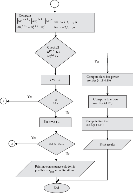
Fig 4.6 Power Flow Study by GS Method – Flow Chart (Contd.)
nob=length(lineinfo(:,1)); n = max(max(Fb), max(Tb));
Z = R + j*X; y= ones(nob,1)./Z;
for i = 1:nob
Ybus=zeros(n,n);
for k=1:nob;
Ybus(Fb(k),Tb(k))=Ybus(Fb(k),Tb(k))–y(k);
Ybus(Tb(k),Fb(k))=Ybus(Fb(k),Tb(k));
end
end
for i=1:n
for k=1:nob
if Fb(k)==i
Ybus(i,i) = Ybus(i,i)+y(k) + hlc(k);
elseif Tb(k)==i
Ybus(i,i) = Ybus(i,i)+y(k) +hlc(k);
else, end
end
end
n = length(businfo(:,1));
for a=1:n
bn=businfo(a,1);
bustype(bn)=businfo(a,2); Vmag(bn)=businfo(a,3);
Vang(bn)=pi/180*businfo(a, 4);
Pd(bn)=businfo(a,5); Qd(bn)=businfo(a,6); Pg(bn)=businfo(a,7); Qg(bn) = businfo(a,8);
Qmin(bn)=businfo(a, 9); Qmax(bn)=businfo(a, 10);
V(bn) = Vmag(bn)*(cos(Vang(bn)) + j*sin(Vang(bn)));
P(bn)=(Pg(bn)–Pd(bn))/MVAb;Q(bn)=(Qg(bn)–Qd(bn))/MVAb;
end
conv = 1;
Vcal = zeros(n,1)+j*zeros(n,1); Scal = zeros(n,1)+j*zeros(n,1);
iter=1;
maxerr=10;
while maxerr >= error & iter <= maxiter
for i = 1:n;
if bustype(i) ~= 1
YV = 0+j*0;
for k = 1:n;
if i~=k & Ybus(i,k)~=0;
YV = YV + Ybus(i,k)*V(k);
end
end
Scal = conj(V(i))*(Ybus(i,i)*V(i) + YV) ;
Scal = conj(Scal);
if bustype(i) == 2
Q(i) = imag(Scal);
Qgcal = Q(i)*MVAb + Qd(i) ;
x=0;
if Qgcal < Qmin(i),
Q(i) = Qmin(i); x=x+1;
elseif Qgcal > Qmax(i),
Q(i) = Qmax(i); x=x+1;
end
end
Vcal(i) = ((P(i)–j*Q(i))/conj(V(i)) — YV )/ Ybus(i,i);
if bustype(i) == 2
if x==1
Vmag(i)=abs(Vcal(i));
else,end
Vcal(i)= Vmag(i)*[cos(angle(Vcal(i)))+j*sin(angle(Vcal(i)))];
else,end
V2(i) = V(i) + accel*(Vcal(i) –V(i));
DVmag(i) = abs(V(i)) – abs(V2(i));
DVang(i) = angle(V(i)) – angle(V2(i));
V(i)=V2(i);
end % end of if
end % end of for
maxerr=max( max(abs(DVmag)), max(abs(DVang)) );
if iter == maxiter & maxerr > error
conv = 0;
else, end
iter=iter+1;
end
for i = 1:n
Vmag(i) = abs(V(i)); Vangrd(i) = angle(V(i))*180/pi;
if bustype(i)==1
Scal=0;
for k=1:n
Scal = Scal+conj(V(i))*(Ybus(i,k)*V(k) );
end
P(i) = real(Scal); Q(i) = –imag(Scal);
Pg(i) = P(i)*MVAb + Pd(i);
Qg(i) = Q(i)*MVAb + Qd(i);
elseif bustype(i) ==2
Qg(i) = Q(i)*MVAb + Qd(i);
end
end
disp (‘ ———————————Ybus——————————— ’)
disp (Ybus)
if conv == 0
fprintf (‘ solution did not converged after %g iterations. ’, (iter–1))
else,
fprintf (‘Power Flow Solution by Gauss–Seidel Method’);
fprintf (‘ No. of Iterations = %g ’, (iter–1))
end
disp (‘Bus Voltage Angle in —————Load———— ———Generation—— ‘)
disp (‘No. Magnitude Degrees P Q P Q ')
for i=1:n
fprintf (‘ %5g’, i), fprintf(‘ %10.3f’, Vmag(i)),
fprintf (‘%11.3f’, Vangrd(i)), fprintf(‘ %9.3f’, Pd(i)),
fprintf (‘%10.3f’, Qd(i)), fprintf(‘ %11.3f’, Pg(i)),
fprintf (‘%11.3f ‘, Qg(i))
end
fprintf (‘ Total ‘)
fprintf (‘%18.3f’, sum(Pd)), fprintf(‘ %10.3f’, sum(Qd)),
fprintf (‘%11.3f’, sum(Pg)), fprintf(‘ %11.3f’, sum(Qg))
fprintf (‘ Line Flow and Losses ’)
fprintf (‘——Line—— Power flow ——Line lossses in—— ’)
fprintf (‘from to MW Mvar MVA MW Mvar ’)
I=zeros(n,n);
for i=1:n
for l=1:n
if i~=l & Ybus(i,l)~=0
if i>l
I(i,l)= –I(l,i);
else
I(i,l)=–Ybus(i,l)*(V(i)–V(l));
end
S(i,l)= V(i)*conj(l(i,l));
S(l,i)= V(l)*conj(–l(i,l));
fprintf (‘%7g’,i),fprintf (‘%5g’,l),fprintf (‘%12.3f’,real(S(i,l))*MVAb)
fprintf (‘%11.3f’,imag(S(i,l)*MVAb)),fprintf(‘%12.3f’,abs(S(i,l))),
fprintf (‘%10.3f’,real(S(i,l)+S(l,i)))
fprintf (‘%9.3f ‘,imag(S(i,l)+S(l,i)))
end
end
end
Example 4.2
(Numerical example for Case–1 study)
Figure 4.7 shows a 5-bus power system. Each line has an impedance of (0.02 + j0.2) per unit Consider the following bus data (all are per unit values). Neglect line charging admittances.
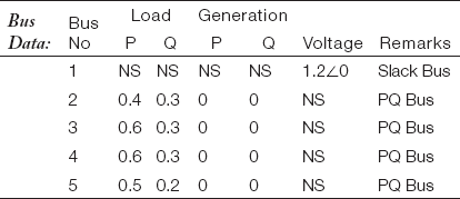
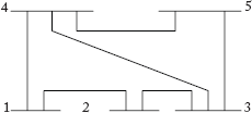
Fig 4.7 5-Bus System for Example 4.2
Form Ybus. Find V2, V3, V4 and V5 after the first iteration using Gauss–Seidel method. Assume flat start (initial voltage values are unity)
Solution:
Series admittance of each line ![]()
Through direct inspection method Ybus is formed and the elements are given below:
Diagonal elements of Ybus
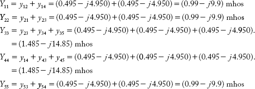
Off-diagonal elements of Ybus:
The Ybus elements in polar form are given below:

b) The injected power at each bus is:
Assume V20 = V30 = V40 = V50 = 1 p.u. and
The first iteration voltages and phase difference are computed below

The first iteration voltage values calculated above are verified with the results obtained by executing the pfstudy_gauss software program.
Convergence Solution is obtained at the end of 18 Iterations.
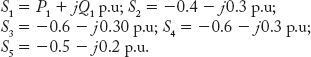
The results are presented below:

Line Flow and Losses
Example 4.3
(Numerical example for Case-2 study)
Consider the 5-bus power system of Example 4.2. Line data remain the same. But, the second bus is now designated as PV Bus.Consider the following bus data.
Bus Data:

Take reactive power limits for PV Bus as –1 ≤ Q2 ≤ 1 p. u.
Find Q2, δ2 V2, V3, V4 and V5 after the first iteration using the Gauss–Seidel method.
Assume flat start (initial voltage values are unity)
Solution:
Since line data is the same as in Example 4.2, the bus admittance matrix is taken.
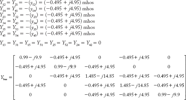
The injected power at each bus is:
S1 = P1 + jQ1 p.u; S2 = 0.5 + jQ2 p.u.
S3 = –0.6 –j0.30 p.u.; S4 = –0.6 –j0.3 p.u.; S5 = –0.5 –j0.2 p.u.
Assume V30 = V40 = V50 = 1p.u. and
δ40 = δ30 = δ40 = δ50 = ![]() 0
0
Given that V20= 1.1 + j0, |V2|=1.1;
Using Equation 4.27, Q21 is calculated as:

The value of Q21 is within the imposed limits of Q2 min and Q2 max.
Using the above value of Q21, we find V21 as

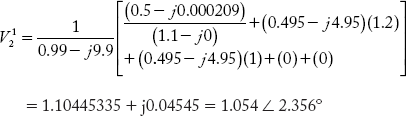
Therefore, δ12 = 2.356°
We set ![]() , and retain the phase angle
, and retain the phase angle ![]() . Thus, the value of
. Thus, the value of ![]() for subsequent iteration is set to
for subsequent iteration is set to ![]() = 1.1
= 1.1 ![]() 2.356°
2.356°

The first iteration voltage values calculated above are verified with the results obtained by executing pfstudy_gauss software program.
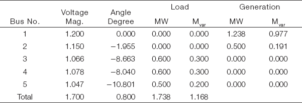
Convergence Solution is obtained at the end of 20 iterations.
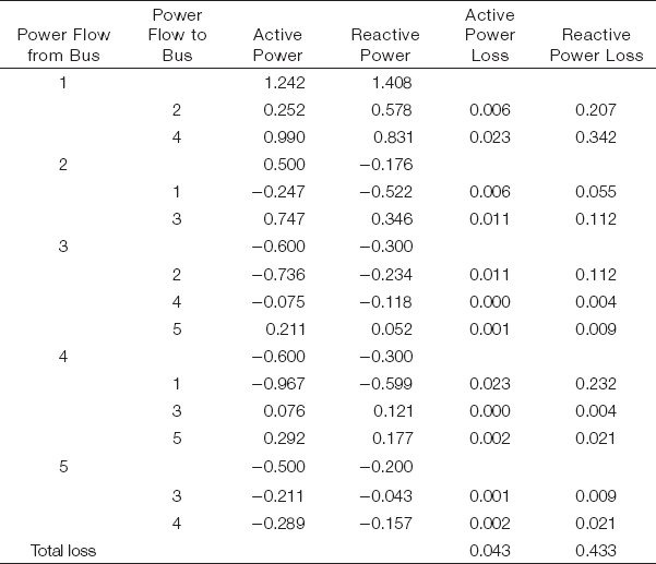
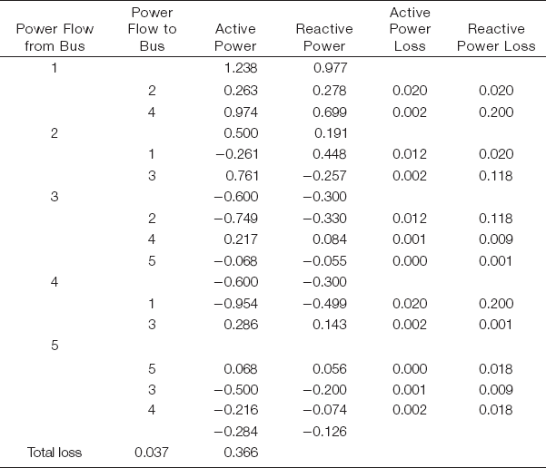
The results are presented below:

Power Flow and Losses
Example 4.4
(Numerical example for the case when the PV bus Q value violates limits)
In Example 4.3, the reactive power limits are changed to new limits as: 0.3 ≤ Q ≤ 0.1 p.u. Execute pfstudy_gauss software and observe how Bus-2 is re-designated as PQ bus.
Obtain final bus voltages.
Convergence Solution
The pfstudy_gauss software program results at the end of 39 iterations
Power Flow and Losses
Example 4.5
(Numerical example for slack bus power calculations)
Consider a 2-Bus power system shown in Figure 4.8. The loads at the buses are shown in the figure. The Ybus of the network is
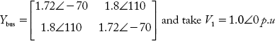
Using second iteration value of V2, calculate injected powers at the first bus.

Fig 4.8 2-Bus Power System of Example 4.5
Solution:
The power into the buses is
Let us have a flat start for V2
Now the first iteration value of V2 is:

The next iteration yields,

Substituting the above values
With k = 1, the above expression yields the complex power for Bus 1;
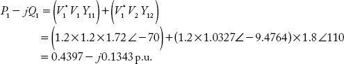
From the above,
P1 = 0.4397 p. u., Q1 = 0.1343 p. u.
Example 4.6
(Numerical Example for use of acceleration factor)
The following Figure 4.9 shows a 3-Bus power system. The line and bus data are given in p. u.
Neglect line charging admittances.

Fig 4.9 3-Bus Power System of Example 4.6
| Line Between buses | Series admittance |
|---|---|
| 1 – 2 | 2 – j8 |
| 1 – 3 | 1 – j5 |
| 2 – 3 | 1 – j4 |
Form Ybus, and compute voltages at buses 2 and 3 at the end of the first iteration. Take acceleration factor as 1.6.
Use flat start.
Solution:
The line admittances and power injected into various buses are shown. The elements of the bus admittance matrix are:


Assume V20 = V30 =1![]() 0°;
0°;
Using Eq. (4.20) V21 and V31 are calculated as below
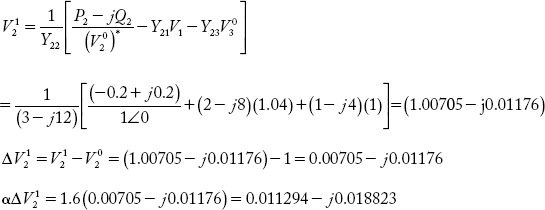
Accelerated V21 = V20 + α ∆ V21 = 1.011294 – j0.018823

Accelerated V3 = V30 + (α ∆ V31) = 0.98923 –j0.01965
4.8 Conclusion
In this chapter, power flow solution by the Gauss—Seidel method was described. The method is simple and is suitable for small-sized power systems. The technique has been elaborated upon using a flow chart, and adequate numerical examples have been provided to help the reader understand the concept. The MATLAB program pfstudy_gauss for the method is presented along with the test results of the standard IEEE bus systems.
Questions from Previous Question Papers
- Explain the significance of power flow studies.
- Describe data preparation power flow studies.
- Describe the applications of power flow studies.
- Derive the static load flow equations and comment on the same.
- Why are buses classified?
- How are buses classified?
- Explain the Gauss—Seidel Method.
- Why is acceleration factor used in the GS Method?
- Give your comments on the GS Method
- Explain the significance of slack bus.
- Explain the significance of voltage-controlled buses.
- What steps must be taken if the reactive power limits of a PV bus is violated?
- A power flow solution is possible without PV Buses. Explain how.
- Give the algorithm for power flow solution by the GS Method.
- Develop a flow chart for power flow solution by the GS Method.
- Classify the various types of buses and explain the necessity of load flow studies.
- Write short notes on data for power flow studies
(Or)
Explain the terms PQ, PV and slack buses for a power system and indicate their significance.
- Derive static load flow equations.
- Write short notes on choice of acceleration factors (Or) What are acceleration factors? Explain their importance in power flow studies.
- Explain the load flow solution using Gauss—Seidel Method with the help of a flow chart
- Describe load flow solution with PV busses using G-S Method.
- Draw flow chart for load flow solution by GS Method using YBus. What are PV buses? How are they handled in the GS Method.
- Explain why often use YBus rather than ZBus in the load flow studies.
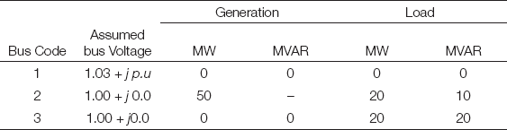
- The load flow data for the power system shown in Figure Q1 is given in the following tables
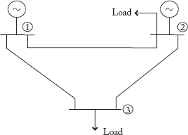
Fig Q1
The voltage magnitude at bus (2) is to be maintained at 1.03 p.u. The maximum and minimum reactive power limits of the generator at bus (2) are 35 and 0 MVAR respectively, with Bus 1 as slack bus. Obtain voltage at bus (3) using GS Method after first iteration (Assume base MVA = 50)
Line Data:
Bus Code p – q Impendance Zpq 1–2 0.08 1 j0.24 1–3 0.02 1 j0.06 2–3 0.06 1 j0.18 Bus Data:

- The load flow data for the system shown in Figure Q2 is given below in the following tables.

Fig Q2
Line Data:
Bus Code p–q Inpedence Zpq 1–2 0 + j0.05 pu 1–3 0 + j0.1 pu 2–3 0 + j0.05 pu Bus Data:
The voltage magnitude at bus (2) is to be held at 1.0 p.u. The maximum and minimum reactive power limits at bus (2) are 50 and 10 MVAR respectively. With bus (1) as the slack, use GS Method and YBus to obtain a load flow solution upto one iteration.
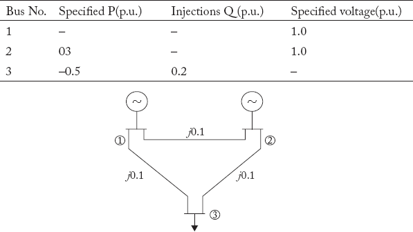
- Consider the 3-bus system shown in Figure Q3. The p.u. line reactances are indicated on the figure. The line reactances are negligible. The magnitude of all the 3-bus voltages are specified to be 1.0 p.u. The bus powers are specified in the following table.
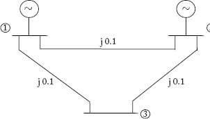
Fig Q3
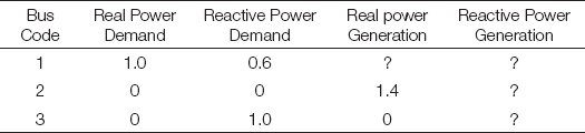
? indicates that the quantity is unspecified. All numerical values are expressed as p.u. values.
- A 2-Bus system is shown in Figure Q4. Determine the voltage at bus (2) by GS Method after 2 iterations.
The YBus elements are:
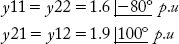
and bus(1) voltage V1 = 1.1
 p.u.
p.u.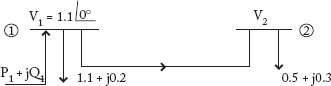
Fig Q4
- The data for a 2-bus system is given below:
SG1 = unknown; SD1 = unknown
V1 = 1.0
p.u.; S1 = To be determinedSG2 = 0.25 + jQ G2 p.u; SD2 = 1 + j0.5 p.u.
The two buses are connected by a transmission line of p.u. reactance of 0.5 p.u. Find Q2 and magnitude of V2. Neglect shunt susceptance of the tie line. Assume V2 = 1.0 p.u. perform two iterations using GS Method.
Competitive Examination Questions
- In load flow studies of a power system, the quantities specified at a voltage controlled bus are ________ and ________.
[GATE 1992 Q.No. 4]
- In load flow analysis, the load connected at a bus is represented as
- constant current drawn from the bus
- constant impedance connected at the bus
- voltage and frequency dependent source at the bus
- constant real and reactive drawn from the bus
[GATE 1993 Q.No. 4]
- If the reference bus is changed in two load-flow runs with the same system data and power obtained for reference bus taken as specified P and Q in the latter run,
- the system losses will be unchanged but complex bus voltages will change
- the system losses will change but complex bus voltages remain unchanged
- the system losses as well as complex bus voltage will change
- the system losses as well as complex bus voltage will be unchanged
[GATE 1995 Q.No. 2]
- Using Gauss–Seidel load flow method, find the bus voltages at the end of one interaction for the following 2 bus system. Line reactances are shown in figure. Ignore resistance and line charging. Assume initial voltage at all buses to be 1.0<0. Use 1.0 as acceleration factor. The bus data is given in the table below.
[GATE 1996 Q.No. 11]
- Gauss–Seidel iterative method can be used for solving a set of
- linear differential equations only
- linear algebraic equations only
- both linear and nonlinear algebraic equations
- both linear and nonlinear differential equations
[GATE 1997 Q.No. 1]
- In load flow studies of a power system, the quantities specified at a voltage controlled bus are ________ and ________.
[GATE 1997 Q.No. 7]
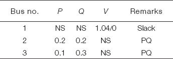
- In a 3-bus system, Gauss load flow method is to be used for finding the switched capacitor compensation required to maintain the voltage at bus 2 equal to 1.0 p.u. the data for the system is as follows:
Bus data:
Bus No. Bus Type Specifications 1 Slack V1 = (1 + j0) p.u. 2 PV Load: P2 + jQ2 = (0.4 + j0.2)p.u. V2 (maganitude) = 1.0p.u. 3 PQ Load: P3 + jQ3 = (0.3 + j0.15)p.u. All data are on common base values.
With the help of one iteration of load flow, explain how will achieve the stated objective.
[GATE 2000 Q.No. 12]
- A power system consists of 2 areas (Area 1 and Area 2) connected by a single tie line (figure). It is required to carry out a load flow study on this system. While entering the network data, the tie-line data (connectivity and parameters) is inadvertently left out. If the load flow program is run with this incomplete data,
- the load-flow will converge only if the slack bus is specified in Area 1
- the load-flow will converge only if the slack bus is specified in Area 2
- the load-flow converge only if the slack bus is specified in either Area 1 or Area 2
- the load-flow will not converge if only one slack bus is specified.
[GATE 2002 Q.No. 5]
- A power system consists of 300 buses out of which 20 buses are generator buses, 25 buses are the ones with reactive power support abd 15 busses are the ones with fixed shunt capacitors. All the other buses are load buses. It is proposed to perform a load flow analysis for the system using Newton–Raphson method. The size of the Newton–Raphson Jacobian matrix is
- 553 × 553
- 540 × 540
- 555 × 555
- 554 × 554
[GATE 2003 Q.No. 2]
- The Gauss–Seidel load flow method has following method has following disadvantages. Tick the incorrect statement
- Unreliable convergence
- Slow convergence
- Choice of slack bus affects convergence
- A good initial guess for voltages is essential for convergence
[GATE 2006 Q.No. 9]
- For the Y-bus matrix of a 4-bus system given in per unit, the buses having shunt elements are
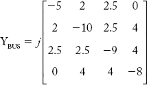
[GATE 2009 Q.No. 26]
- An interconnector cable having a reactance of j0.05 pu links two generating stations G1 and G2 as shown in the figure below, where | V1|=|V2|=1 pu. The load demands at two buses are SD1 = 15 + j5 pu and SD2 = 25 + j15 pu. The total reactive power (in pu) at the generating station G1 when δ = 15o is
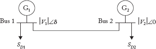
- 25.68
- 25
- 5.68
- 5
[JTO 2009 Section II, Q.No. 33]