
CHAPTER 2
Power System Network Matrices—1
2.1 Introduction
Various studies have to be conducted for the analysis of steady state or dynamic state of a power system. As discussed in Chapter 1, a study is unfolded in three stages: network modelling stage, mathematical modelling stage and solution stage.
In the network modelling stage, various components of the power system are represented by their individual electrical equivalents, converting the single-line diagram of the power system network into an electrical network consisting of active and passive elements.
The electrical network model is converted into a suitable mathematical model comprising of algebraic or differential equations for performing network analysis. For the sake of convenience, these network equations are then represented in the form of network matrices. The frame of reference for these network matrices is either a loop or a bus. Nodes in the power system are otherwise known as buses. The bus frame of reference is popularly used by researchers.
Finally, in the solution stage, the network equations are solved by using appropriate numerical techniques for the purpose of system analysis.
The usage of power system network is widespread and complex, dealing with the interconnection of a large number of components. For such large complicated networks, network equations may be formulated easily by applying the graph theory or network topology. In this chapter, we discuss the formulation of network equations and matrices using topological techniques, while the building algorithms needed for such formulations are examined in Chapter 3.
2.2 Graph of a Power System Network
A graph represents the geometrical structure of a power system network. In other words, it describes how various power system components are interconnected to form a network. In the graph, components are represented as line segments. Consider the following example to understand the significance of the graph theory. Three network segments extracted from three different networks and their structure is represented by a graph, as shown in Figure 2.1.
It may be seen from Figure 2.1 that the same network equation I3 = I2 + I1 can be obtained by applying KCL to the junction node in the three segments shown in Figure 2.1 (i – iii), as well as in the graph (Figure 2.1(iv)). This means that network equations developed based on either KCL or KVL do not depend on the type of elements (such as R, L, C) but rather on the structure of the network. Since the structure of the three segments is similar to that in Figure 2.1(iv), the same network equation is obtained. This process simplifies working with complicated networks since we merely use the network structure to formulate network equations. Topological and graphical techniques form the basis of using the computer in network analysis.
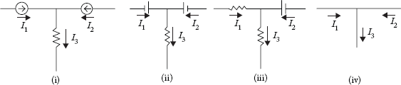
Fig 2.1 Three Segments Extracted From Three Different Networks and Their Representation as a Graph
2.3 Definitions
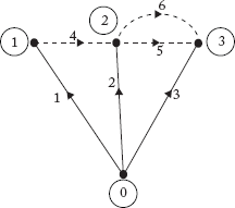
In this section, we look at some of the definitions related to the usage of graphs in power system analysis. Consider the power system network of Figure 2.2. It has six components, namely, three generators G1, G2 and G3, one transformer T1 and two transmission lines L1 and L2.
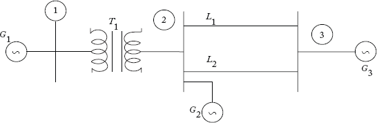
Fig 2.2 A Typical Power System Network
2.3.1 Graph
In a graph, each element of the power system is represented as a line segment, connecting any two nodes or buses. Figure 2.3 shows the graph of the power system network depicted in Figure 2.2. Note that the generator is connected between the reference node (0) and other nodes. In the graph, node numbers are circled, while element numbers are not circled.
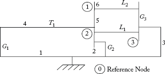
Fig 2.3 Graph of the Power System Network Shown in Figure 2.2
The shape of the graph may be different, but the structure remains the same. For example, the graph of Figure 2.3 is shown differently in Figure 2.4.
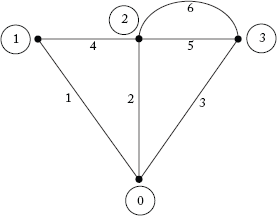
Fig 2.4 A Different Shape of the Graph Shown in Figure 2.3
2.3.2 Planar and Non-Planar Graphs
If the line segments in the graph are not criss-crossing each other, then the graph is said to be planar (or linear); otherwise, it is a non-planar graph.
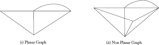
Fig 2.5 Planar and Non-Planar Graphs
2.3.3 Rank of a Graph
The rank of a graph consisting of n number of nodes is (n – 1), the rank of the graph shown in Figure 2.4 is 3.
2.3.4 Oriented Graph
If the line segments of the graph are assigned some arbitrary direction, then it is known as an oriented graph. The arrows on the elements indicate the orientation of the elements. Elements whose ends fall on a node are said to be incident at the node. In Figure 2.6, elements 2, 4, 5 and 6 are incident at node 2.
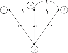
Fig 2.6 Oriented Graph of the Graph Shown in Figure 2.4
2.3.5 Sub-Graph
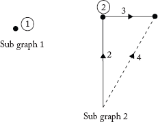
A sub-graph is a subset of the buses and elements of a graph. Figure 2.7 represents a few sub-graphs of the graph shown in Figure 2.6.
2.3.6 Path
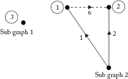
A path is a sub-graph of connected elements, with not more than two elements connected at internal nodes. However, at the two terminal nodes, only one element is connected. Figure 2.8 represents the paths of the graph shown in Figure 2.6.
2.3.7 Connected Graph
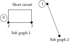
A graph or sub-graph is said to be connected when there exists at least one path between any two nodes. Figure 2.9 represents the connected/unconnected sub-graphs of the graph shown in Figure 2.6.
2.3.8 Tree
A tree is a connected sub-graph of a connected graph having all the nodes of the graph, but without any closed loop. The elements of a tree are called ‘branches’ or ‘twigs’. Figure 2.10 represents a few possible trees of the graph shown in Figure 2.6. The rank of a tree is the same as that of its parent graph.
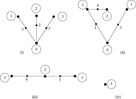
Fig 2.7 Sub-Graphs of the Graph Shown in Figure 2.6
Note: Some sub-graphs may contain a single node of the original graph (see Figure 2.7(iv)).
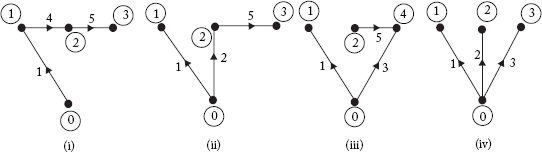
Fig 2.8 Paths of the Graph Shown in Figure 2.6
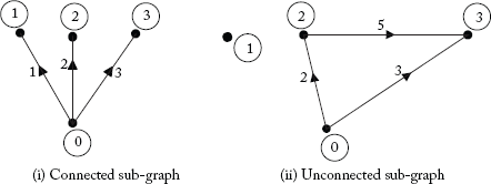
Fig 2.9 Connected/Unconnected Sub-Graphs of the Graph in Figure 2.6
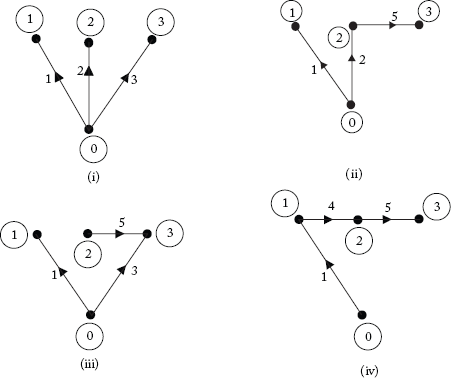
Fig 2.10 Some Possible Trees of the Graph Shown in Figure 2.6
Note: In Figure 2.10(i), all branches are incident at the reference or common node (0). Such trees are called star trees. Star trees are preferred for convenience.
2.3.9 Co-Tree
A co-tree is the complement of a tree and is a sub-graph of the graph formed with the elements other than those in the tree. Co-tree elements are called links or chords.
Usually, the branches (twigs) of a tree are represented by dark lines, whereas links (chords) are represented by dashed lines as shown in Figure 2.12.
Let, e = total number elements in a graph, n = total number of nodes, b = total number of branches and l = total number of links.
Then b = n – 1 and l = e – b = e – (n – 1) = e – n + 1.
In general, a tree is a connected sub-graph and the co-tree is not necessarily connected.
2.3.10 Basic Loops or Fundamental f-Loops
Whenever a link element is added to the existing tree, Basic loops or fundamental f-loops can be obtained.
The f-loops for the graph in Figure 2.12 are shown in Figure 2.13.
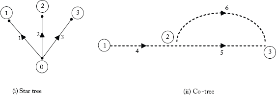
Fig 2.11 Star Tree and Co-Tree of the Graph Shown in Figure 2.6
Note: Tree + Co-Tree = Graph

Fig 2.12 Linear Graph of the Network Shown in Figure 2.6
The orientation of the f-loops is assumed to be the same as that of the link, which is added to obtain the f-loop.
Note: Number of f-loops = Number of links.
2.3.11 Basic Cutsets or Fundamental f-Cutsets
A basic or fundamental f-cutset of a graph is the set of elements consisting of only one branch (or twig) and a minimal number of links (or chords). When these sets of elements are removed from the graph, the graph will be divided exactly into two unconnected sub-graphs. Due to the removal of cutset elements, one of the two resulting sub-graphs will consist of an isolated node.
The basic cutsets of the graph in Figure 2.12 are shown in Figure 2.14.
Note: Number of basic cutsets 5 Number of branches.
All the f-cutsets of the graph in Figure 2.12 are marked in Figure 2.15. The orientation of f-cutsets is the same as that of the branch.
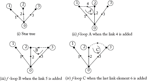
Fig 2.13 The Basic or f-Loops of the Graph in Figure 2.12

Fig 2.14 Basic or f-Cutsets of the Graph in Figure 2.12
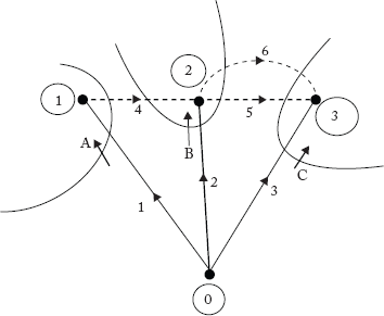
Fig 2.15 Diagram Showing all the Basic or f-Cutsets of the Graph in Figure 2.12
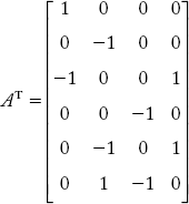
The number of possible trees that can be constructed from a graph can be obtained by using the following formula.
If AT is the transpose of A matrix then the number of trees of a given graph = determinant [AT.A]
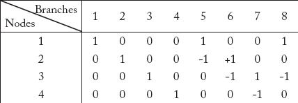
2.4 Incidence Matrices
Every element of a graph is incident between any two nodes. Incidence Matrices give the information about the incidence of elements to nodes and their orientation with respect to nodes. The elements may be incident to loops, cutsets or other such parts of a graph. This information is furnished in the incidence matrix. Various types of incidence matrices are presented in the following sections.
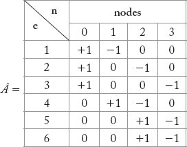
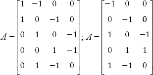
2.4.1 Element Node Incidence Matrix [Â]
This incidence matrix (Â) describes whether an element is incident to a particular node or not. Any general entry aij of the matrix (Â) can be entered as in Table 2.1.
The dimension of the matrix  is e × n.
In matrix  the entries 1 and –1 for a particular element occur in pair and other entries for the element are zero. Consequently, the sum of the elements in a row of Â, is zero, indicating that one column of  is the negative sum of other columns, and can therefore be eliminated. The rank of  is thus (n – 1).
Table 2.1 General Entry of an Element in Matrix (Â)
| aij (ith row and jth column element) | = 1, if the jth element is incident to the jth node, and oriented away from the jth node. |
| = –1, if the jth element is incident to the jth node, and oriented towards the jth node. | |
| = 0, if the element is not incident to the jth node. |
Example 2.1
Obtain  matrix for the graph shown in Figure 2.12
Solution:
The  matrix for the graph shown in Figure 2.12 has been formed by following conventions as in Table-2.1 and is given below:
2.4.2 Bus Incidence Matrix [A]
This matrix A is obtained from  upon elimination of the column corresponding to the reference node 0.
Example 2.2
Obtain the A matrix for the graph shown in Figure 2.12
Solution:
Upon removing the first column corresponding to reference node 0, the A matrix is obtained and is given below:
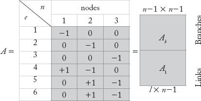
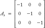
The A matrix can be partitioned into two sub-matrices: Since the number of branch elements b = n – 1, the sub-matrix Ab is a square matrix. The sub-matrix Ab is a non-singular square matrix with rank (n – 1).
Application of A matrix:
The matrix A is useful in formulating network equations such as those for voltage drop of the individual elements (branch voltages), expressed in terms of node voltages. Example 2.3 demonstrates this feature.
Example 2.3
Using the graph in Figure 2.12, develop the equations for branch voltages in terms of node voltages. Assume that the reference node voltage is zero.
Solution:
Let the node voltages be v1, v2 and v3 and reference node voltage. V0 = 0. The v's represent voltage drops in the individual elements. Assuming the orientation of the element in the graph as the direction of current, the expressions for branch voltages are as follows:
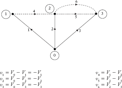
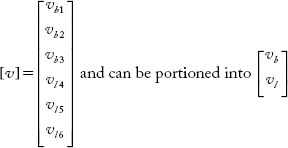
The above equations can be written in the form of the following matrix:
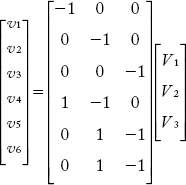
It can be observed that [A] matrix obtained in this example is the same as the matrix obtained in Example 2.1. Therefore, the above matrices can be written in a condensed form as:
where
[v] is the e × 1 column matrix representing branch voltages.
[A] is the e × (n – 1) bus incidence matrix.
[V] is the (n – 1) × 1 column matrix representing node voltages.
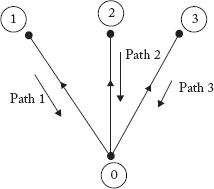
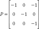
2.4.3 Branch Path Incidence Matrix [P]
Whenever a branch element is added, a new node is created. A path is defined as the set of elements that are present between the newly created node and the reference node-0. The orientation of the path is from the newly created node to the reference node.
Note:
Number of paths = Number of branch elements.
The procedure to obtain paths for the graph shown in Figure 2.12 is illustrated below:
Step 1: Start from reference node 0, add branch element 1 to create a new node 1
Step 2: Add branch element 2, to create a new node 2.
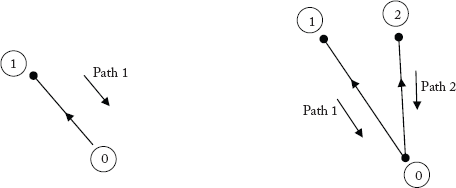
Step 3: Add branch element 3, to create a new node 3.
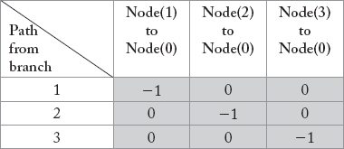
The matrix branch path incidence matrix (P) furnishes information about the incidence of branches in the paths of a tree. Any general entry in the matrix Pij can be entered as in Table 2.2.
Table 2.2 General entry of an element in the branch path incidence matrix
| Pij = (ith row – jth column element) | 1, if the ith branch is in the path from the jth node to the reference node (0) and oriented in the same direction of the path. |
| 1, if the ith branch is in the path from the jth node to the reference node and oriented in the same direction of the path. | |
| 0, if the ith element is not in the path from the jth node to the reference node. |
Example 2.4
Obtain the P matrix for the graph shown in Figure 2.12
Solution:
The branch path incidence matrix (P) of the graph in Figure 2.12 is given below.
The matrix P is a non-singular square matrix with rank (n – 1).
Relation between matrices Ab and P
Consider the matrices A and P obtained for the graph shown in Figure 2.12.
The sub-matrix Ab of the incidence matrix A describes the incidence of branch to nodes and is given by:
The matrix P describes branches to paths and is given by:
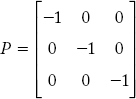
Since there is a relation between the paths and buses, we can prove the relation AbT P = U, where U is the identity matrix.
By using the above matrices the relation is verified as follows:
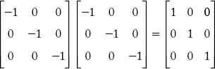
Since
we can write
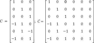
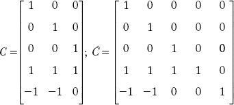
2.4.4 Basic Cutset (or) Fundamental Cutset Incidence Matrix [C]
The basic cutset (or) f-cutset incidence matrix (C) gives information about the incidence of elements in a particular f-cutset.
Any ith row, jth column element Cij of the matrix can be entered as shown in Table 2.3.
Table 2.3 General entry of element in the matrix P
| Cij = | 1, if the ith element is incident to and oriented in the same direction as the jth f-cutset. |
| 1, if the ith the element is incident to and oriented in the opposite direction as the jth f-cutset. | |
| 0, if the ith element is not incident to the jth f-cutset. |
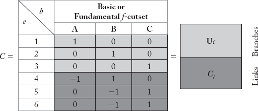
The dimension of [C] matrix is e * b, where e is the number of elements and b is the number of branches.
The [C] matrix for the graph shown in Figure 2.12 is formed by following the conventions mentioned in Table 2.3 and is as given below:
Application of C-matrix:
Network equations can be developed based on KCL using the C-matrix. Consider the graph in Figure 2.15.
Let Ii, i = 1, 2, …, 6, be the current flowing through individual elements.
Applying KCL at nodes 1, 2 and 3, the following equations can be obtained:
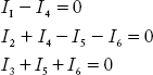
The same equations can be obtained from the following equation:
where CT is the transpose of the f-cutset incidence matrix and [I] is the column matrix containing element currents. The dimensions of CT and [I] matrices are [b × e] and [e × 1] respectively.
Note:
Number of network equations based on KCL = number of f-cutsets
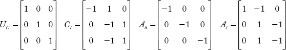
The matrix C can be partitioned into two subsets UC and Cl of sizes (b × b) and (l × b) respectively, where UC is the identity matrix.
It may be noted that:
- The identity matrix UC describes the incidence of branches to f-cutsets.
- The sub-matrix Cl relates the links to the f-cutsets (or to the isolated node).
- The sub-matrix Ab relates incidence of branches to nodes.
- The sub-matrix Al relates incidence of links to nodes.
From the above observations it may be concluded that there is a one-to-one correspondence between branches and f-cutsets and links to the f-cutsets, and the following relation may be developed:

Equation (2.4) may be verified with the incidence matrices obtained earlier for the graph in Figure 2.12 and is illustrated below.
The partitioned sub-matrices of Ab, Al and Cl for the graph shown in Figure 2.12 are:
Now we have to verify the relation Cl Ab = Al

From the above it is proved that, Cl Ab = Al
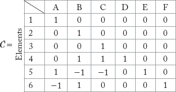
2.4.5 Augmented or Tie Cutset Incidence Matrix [Ĉ]
The matrix C is of size e × b. Therefore, it is a non-square matrix and its inverse does not exist. In other words, C is a singular matrix. In order to make the matrix C a non-singular matrix, we augment it with a number of columns that equals the number of links by adding fictitious cutsets known as tie cutsets, which contain only the links. The tie cutsets are added to the graph in Figure 2.12 and are shown in Figure 2.16.
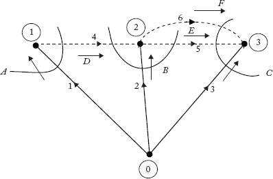
Fig 2.16 Graph Showing Tie Cutsets D, E, F and f- Cutsets A, B, C
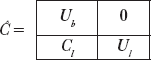
Now, the augmented cutset incidence matrix Ĉ can be represented as shown:
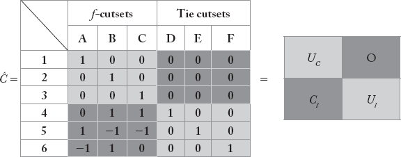
The matrix Ĉ can be partitioned into four sub-matrices: null matrix [0] of size b × l, identity matrix Ul of size l × l, UC and Cl as described earlier.
Example 2.5
Obtain Ĉ matrix for the graph shown in Figure 2.17(a).
Solution:
In the example,
e = 6, n = 4, b = 4 – 1 = 3, and l = 6– 4 + 1 = 3
Therefore, number of basic cutsets = b = 3 and number of tie cutsets = l = 3
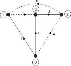
Fig 2.17(a) Graph for Example 2.5
Note that the tree of the graph is not a star tree.
Through the following steps, we shall develop f-cutsets
Step 1: Isolate node 1
By removing branch 1and links 5 and 6, node 1 is isolated.
Therefore cutset A = {1, 5, 6}
Step 2: Isolate node 2
To isolate node 2 from other nodes, branch 2 and link 6 can be removed. However, element 3 cannot be removed as it is a branch element. Hence to isolate node 2 it is required to isolate node 3. This can be understood in such a way that node 2 is short circuited with node 3. To isolate node 3 (which is short-circuited to node 2), elements 4 and 5 need to be removed.
Therefore f-cutset B = {2, 4, 5, 6}
Step-3: Isolate node 3.
By removing branch 3 and links 4 and 5, node 3 is isolated. Therefore cutset C = {1, 5, 6}
f-cutset C = {3, 4, 5}. Now, the tie cutsets are D = {4}, E = {5} and F 5{6}.

Fig 2.17(b) Graph Showing f-cutsets and Tie Cutsets of the Graph Shown in Figure 2.17(a)
All the cut sets are shown in Figure 2.17(b).
The augmented or tie-cut set incidence matrix Ĉ is given by
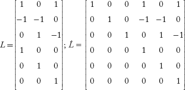
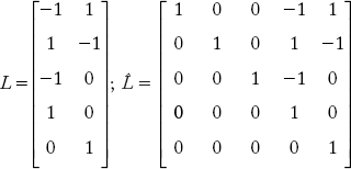
2.4.6 Basic or Fundamental f -loop Incidence Matrix [L]
Whenever a link element is added, a new basic or fundamental f-loop is created. The number of f-loops is equal to number of links. The f-loop incidence matrix L depicts the incidence of an element in a particular f-loop. Any ith row, kth column element of an L matrix can be entered as described in Table-2.4.
Table 2.4 General entry of element in the matrix L
| Lik = | 1, if the ith element is incident in the kth f-loop and oriented in the same 1, 1, if the ith element is incident in the kth f-loop and oriented in the same direction. |
| –1, if the ith element is incident in the kth f-loop and oriented in the opposite direction. | |
| 0, if the ith element is not incident in the kth f-loop. |
Example: 2.6
Obtain L matrix for the graph shown in Figure 2.12
The f-loops A, B and C for the graph in Figure 2.12 are shown in Figure 2.18. By following conventions mentioned in the Table 2.4, the L-matrix is obtained and is given below:
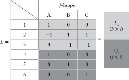
The loop incidence matrix L is divided into two sub-matrices Lb and Ul as shown above.
2.4.7 Augmented Loop Incidence Matrix 
The matrix L is not a square matrix and hence it is a singular matrix. By adding b number of fictitious open loops to the L matrix, it can be converted to a square matrix, and is known as augmented loop incidence matrix ![]() . An open loop is the path between adjacent nodes connected by a branch. The orientation of the b number of open loops is the same as that of their respective branches. For the graph shown in Figure 2.12 f-loops (A, B, C) and open loops (D, E, and F) are shown in Figure 2.18.
. An open loop is the path between adjacent nodes connected by a branch. The orientation of the b number of open loops is the same as that of their respective branches. For the graph shown in Figure 2.12 f-loops (A, B, C) and open loops (D, E, and F) are shown in Figure 2.18.

Fig 2.18 Graph Showing f-Loops and Open Loops of the Graph Shown in Figure 2.12
The augmented loop incidence matrix for the graph shown in Figure 2.12, with reference to Figure 2.18 can be obtained as:

Example 2.7
For the network shown in Figure 2.19(a) draw the oriented graph and formulate the following: element node incidence matrix, bus incidence matrix, basic cut set incidence matrix, augmented cut set incidence matrix, basic loop incidence matrix, augmented loop incidence matrix and branch path incidence matrix.
Solution:
Oriented graph for the network in Figure 2.19(a) is shown in Figure 2.19(b).
From the oriented graph,
No. of elements (e) = 6
No. of nodes (n) = 4
No. of branches (b) = 3
No. of links (e – b) = 3
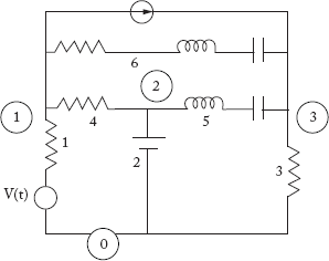
Fig 2.19(a) Network for Example 2.7
Note: The current source in the graph is represented by an open circuit. Hence it is not considered in the graph.
Consider the oriented graph shown in Figure 2.19(b),
Element node incidence matrix (Â) and bus incidence matrix (A):
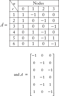

Fig 2.19(b) Oriented Graph of the Network in Figure 2.19(a)
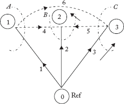
Fig 2.19(c) f-Cutsets of Figure 2.19(a)
The f-cutsets are shown in Figure 2.19(c)
f-cutset A cuts elements = {1, 4, 6}; f-cutset B cuts elements = {2, 4, 5}
f-cutset C cuts elements = {3, 5, 6};
Basic cutset incidence matrix (C) and augmented cutset incidence matrix (Ĉ ):
f- loops and open loops are shown in Figure 2.19(d).
Basic loop incidence matrix (L) and augmented loop incidence matrix (![]() ):
):
Paths are shown in Figure 2.19(e).
Path incidence matrix (P):


Fig 2.19(d) Graph Showing Loops

Fig 2.19(e) Graph Showing Paths
Example 2.8
For the oriented graph shown in Figure 2.20(a), formulate the element node incidence matrix, bus incidence matrix, basic cutset incidence matrix, augmented cutset incidence matrix, basic loop incidence matrix, augmented loop incidence matrix and path incidence matrix.

Fig 2.20(a) Graph for Example 2.8
Solution:
From the oriented graph
No. of elements (e) = 9; No. of nodes (n) = 5; No. of buses = n –1 = 5 –1 = 4; No. of branches = b = n – 1 = 4.
No. of links = e – b = 9 – 4 = 5
Element node incidence matrix and bus incidence matrix:

Basic cut set incidence matrix (C) and augmented cut set incidence matrix (Ĉ):
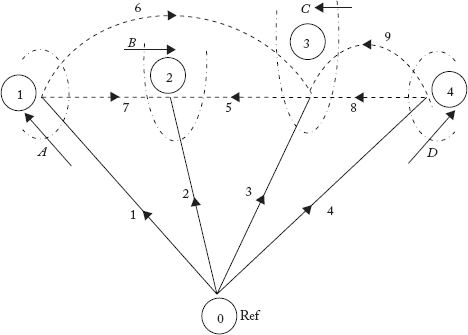
Fig 2.20(b) Graph Showing f-Cutset

Loops are shown in Figure 2.20(c).
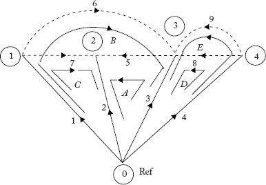
Fig 2.20(c) Graph Showing Loops
Basic loop incidence matrix (L) and Augmented loop incidence matrix (![]() ) are given below:
) are given below:

Paths are shown in Figure 2.20(d). Path incidence matrix (P) is given by:
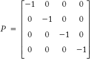
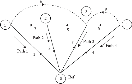
Fig 2.20(d) Graph Showing Paths
2.5 Primitive Network
A power system network consists of a number of elements. Each element is incident between any two nodes. This element may be a purely passive (like z or y), or active (V or I) or a combination of both active and passive.
Each element can be represented by a decoupled partial network, known as the primitive network. This network can be either in admittance or impedance form.
2.5.1 Primitive Network in Impedance Form
Let an element be connected between the two nodes i and k. This is shown in Figure 2.21

Fig 2.21 Primitive Network in the Impedance Form for the Element Connected Between the Two Nodes i and k
Let,
Vi, Vk = ith and kth node voltages respectively
vik = Vi – Vk = voltage across the element i–k
eik = active source of the element i–k
Zik = self impedance of the element i–k
Iik = current flowing through the element i–k
The following performance equation can be written by observing Figure 2.21:
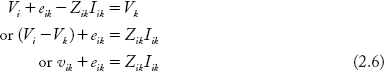
For all elements Equation (2.6) may be written in a condensed form as:
where v, e and I are the column matrices of size e × 1, e is the number of elements and Z is a square matrix of size (e × e). Matrix [Z] is known as the primitive impedance matrix. In general the Z matrix is a diagonal matrix, provided the elements are not mutually coupled to other elements. If the mutual reactance of the elements is given, these can be entered as off-diagonal elements in [Z]. The diagonal elements of [Z] denote self-impedance of the individual elements while the off-diagonal elements stand for mutual impedances.
2.5.2 Primitive Network in Admittance Form
Let the elements i–k be connected between the two nodes i and k. This is shown in Figure 2.22

Fig 2.22 Primitive Network in Admittance Form of Element i–k Connected Between the Nodes i and k
Let
Vi, Vk = ith and kth node voltages respectively.
Vik = Vi – Vk = voltage across the element i–k.
Jik = active current source of the element ik.
yik = self admittance of the element ik.
Iik = current flowing through the element ik.
Now,
Voltage across the element = vik
Current flowing through the element = Iik + Jik
However,
The equation of the type (2.8) for all the elements can be shown in a condensed form as:
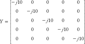
In Equation (2.9), I, J and v are the column matrices of size e × l, and [Y] is a square diagonal matrix of size e × e.
The diagonal elements of [Y] represent self-admittances and off-diagonal elements in [Y] represent mutual admittances of the elements. Off-diagonal elements are zeros if elements have no mutual coupling.
Example 2.9
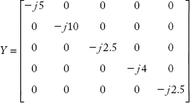
For the network shown in Figure 2.2, give the primitive network matrix in a general form. Assume no elements in the network have mutual coupling.
Solution:
The network consists of six elements. Hence, the dimension of [y] is 6 × 6. In the matrix [y] the diagonal elements are self admittances of individual elements. The suffixes of y indicate the type of element.

Example 2.10
For the power system network shown in Figure 2.23(a),(i) Draw the oriented graph (ii) Formulate the element node incidence matrix, bus incidence matrix, basic cutset incidence matrix, augmented cutset incidence matrix, basic loop incidence matrix, augmented loop incidence matrix, and path incidence matrix (iii) Formulate primitive admittance matrix (take reactance of each element j0.1 p.u).
Solution:
(i) Oriented graph for the network in Figure 2.23(a) is shown in Figure 2.23(b).

Fig 2.23(a) Network for Example 2.10

Fig 2.23(b) Graph for Figure 2.23(a)
(ii) Incidence Matrices
Element node incidence matrix (Â) and bus incidence matrix (A):
From Figure 2.23(a) it can be noted the graph has:
No. of elements (e) = 5; No. of nodes (n) = 4; No. of buses (n – 1) = 3
No. of branches (n – 1) = 3; No. of links (e – b) = 2
Basic cutest incidence matrix (C) and augmented cutset incidence matrix:
f-cutsets: A = {1, 4, 5}; B = {2, 4, 5}; C = {3, 4}
Tie-Sets D = {4}; E = {5}; F = {6}
All cutsets are shown in Figure 2.23(c).
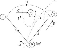
Fig 2.23(c) Graph Showing Cutsets
Basic cutset incidence matrix (C) and augmented cutset incidence matrix are given below:
Basic loop incidence matrix (L) and augmented loop incidence matrix (![]() ):
):
f-loops A, B are shown in Figure 2.23(d)
Branch-path incidence matrix (P):
Paths are indicated in Figure 2.23(e).

Fig 2.23(d) Graph Showing Loops
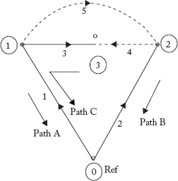
Fig 2.23(e) Paths for the Graph in Figure 2.23(a)
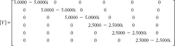
(iii) Primitive admittance matrix:
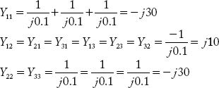
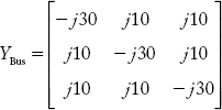
Self-admittance of the Y matrix is: y11 = y22 = y33 = y44 = y55 = 1/j0.1 = –j 10;
The primitive admittance matrix [Y] is:
Example 2.11
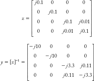
A power system network is shown in Figure 2.24(a). The reactance of each generator is j0.1 p.u and reactance of each line is j0.3 p.u. The two lines have mutual reactance of j0.01 p.u. Formulate the primitive impedance and admittance matrix.
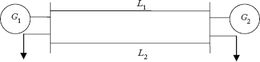
Fig 2.24(a) Network for Example 2.11
Solution:
To find primitive impedance (z) and primitive admittance matrix (y):
Self-impedances: z11 = z22 = j 0.1; z33 = z44 = j 0.3;
Mutual Impedances: z12 = z13 = z14 = z21 = z23 = z24 = 0;
z34 = z43 = j 0.01

Fig 2.24(b) Oriented Graph for Figure 2.24(a)
2.6 Network Equations and Network Matrices
A power system is a large and complex network, which consists of a number of elements such as generators, transformers, transmission lines, controllers, and switching devices. Network analysis or power system analysis requires the development of network equations in a form of network matrices. Though the primitive network describes the characteristics of individual elements it does not provide information about network characteristics such as connections. Therefore we require transforming the primitive network matrices into network matrices. Network matrices can be developed either in the bus frame, branch frame or loop frame of reference. In these frame of references network matrices can be written as:
or
In the above equations, the VBus matrix contains bus voltages, IBus matrix represents injected currents into the buses and ZBus is known as bus impedance matrix for an n-bus power system. The dimensions of these matrices are n × 1, n × 1 and n × n respectively.
The network equations in admittance form can be written as:
where YBus = Z–1Bus
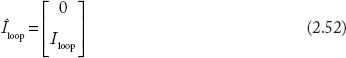
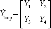
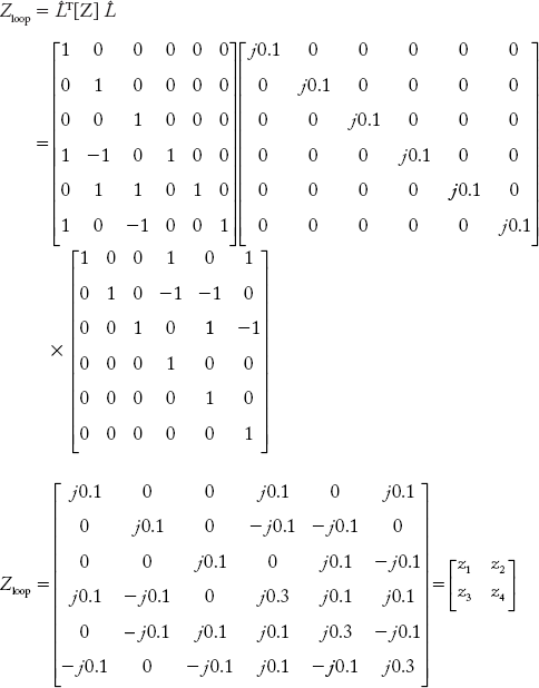
In the loop frame of reference Vloop denotes the basic loop voltages, Iloop represents the basic loop currents and Zloop is the loop impedance matrix. In the admittance form, network equations can be written as:
The size of matrices in the network equation based on loop frame depends on the number of basic loops or links.
Finally, the performance equations can be written in branch frame as:
Here, VBr and YBr represent branch voltages and currents. ZBr and YBr represent branch impedance and branch admittance matrices respectively. The dimensions of these matrices depend upon the number of branches in a graph of a given power system network.
This chapter presents network matrices formulation based on the loop, branch and bus frames. However, the bus frame of reference has emerged as an important frame of reference for developing power system network performance equations, as is evident from recent literature. Studies on power systems like short-circuit studies and power flow studies, are performed by using either the ZBus or the YBus. This frame of reference has advantages like computational convenience and reduced computer memory requirements.
2.7 Bus Admittance Matrix
Bus admittance matrix (YBus) for an n-bus power system is a square matrix of size (n × n). The leading diagonal elements represent the self- or short-circuit driving point admittances with respect to each bus. The off-diagonal elements are the short-circuit transfer admittances or the admittances common to any two buses. In other words, the diagonal element yii of the YBus is the total admittance value with respect to the ith bus and yik is the value of the admittance that is present between the ith and kth buses.
YBus can be obtained through the following methods:
- Direct inspection method
- Step-by-step procedure
- Singular transformation method
- Non-singular transformation method
This section highlights the above methods. The required relations shall be derived in the subsequent sections.
Procedure of forming YBus
Formation of YBus by direct inspection method is suitable for small networks. In this method the YBus matrix is developed by simply inspecting the structure of the network without developing any kind of equations.
The step-by-step procedure is a general-purpose computer algorithm and is similar to the direct inspection method.
In the case of elements having mutual admittances, YBus can be conveniently developed by either singular or non-singular transformation methods. These two methods are based on the graph theory discussed in earlier sections and use of the primitive admittance matrix. Whenever network changes are taking place such as outage of lines or addition of lines, YBus need to be modified. These methods can be easily coded and are quite useful for obtaining the modified YBus.
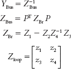
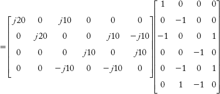
Singular transformation method uses the singular bus incidence matrix A. The equation for YBus in terms of matrix A is:
The method is known as singular transformation method as the matrix A is a singular matrix. The matrix [Y] is a primitive admittance matrix and is discussed in Section 2.4.2.
Non-singular transformation method uses the augmented incidence square matrices. The equation for YBus according to this method is:
where P is the branch path incidence matrix and ZBr is the branch admittance matrix.
The procedure for obtaining YBus using the non-singular transformation method is given below:
Step 1: Form the ZBr matrix by any of the following methods
Method-1:
ZBr = YBr–1 = [CT [y] C]–1 where C is the basic cutset incidence matrix.
Method-2:
ZBr in terms of the non-singular augment cutset incidence matrix Ĉ may be expressed as:
where Ybb, Ylb, Ybl and Yll are partitioned sub-matrices of the primitive admittance matrix [Y] as shown:
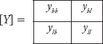
and C1 is a sub-matrix of Ĉ partitioned as:
Method-3:
ZBr = z1 – z2 z4–1 z3
where z1, z2, z3 and z4 are partitioned matrices of the Zloop
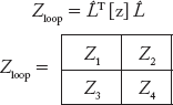
![]() is the augmented loop incidence matrix.
is the augmented loop incidence matrix.
z is the primitive impedance matrix.
Step 2: Now obtain ZBus as:
Step 3: Finally YBus can be obtained as:
All the above methods for YBus formation are discussed in detail in the following sections.
2.7.1 Direct Inspection Method
Consider a 3-bus power system network shown in Figure 2.25. In power flow studies, generators are represented as complex power sources i.e., they are represented by a complex number SGi as:
where SGi = complex power generated at the ith bus,
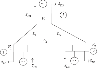
Fig 2.25 A Typical Single Line Diagram Representation of 3-Bus Power System Network
PGi, QGi = active and reactive powers generated at the ith bus.
Loads are represented by a complex number SDi as:
where,
SDi = complex power demand/load at the ith bus
PDi, QDi = active and reactive powers demanded at the ith bus
It may be seen that SGi and SDi denote the local power generation and load respectively at the ith bus. Now, the net power injected into the ith bus Si is the difference of SGi and SDi.
Therefore
Si, Pi, Qi = Complex power, active power and reactive power respectively injected at the ith bus.
Let Vi be the ith bus voltage and
Ii = injected current into the ith bus = IGi – IDi
Now,
Transmission lines are represented as a π-network, with series admittances and two half-line charging admittances. The line connecting buses i and k is represented as a π-network in Figure 2.26.

Fig 2.26 Transmission Line Representation
In Figure 2.26, yik = series admittance of the line i–k
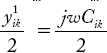
![]() = half-line charging admittance
= half-line charging admittance
Rik, Xik, Cik = resistance, reactance and capacitance of the line i – k
Gik, Bik = conductance and suscpetance of the line i – k
The values of Gik, Bik are obtained as:
The network equivalent of the power system in Figure 2.25 is shown in Figure 2.27.
Applying KCL at junction 1 in Figure 2.28, the equations for net current injected into bus 1 can be written as:
The injected currents in terms of voltages and admittances can be written as:
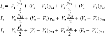
Injected currents can be written as:
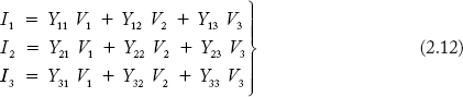

Fig 2.27 Equivalent Circuit of the Power System of Figure 2.21
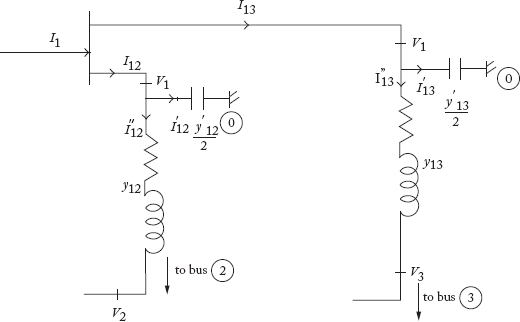
Fig 2.28 Network for Injected Current Calculations
In Equation (2.12),
![]() = total admittance connected to the Bus 1.
= total admittance connected to the Bus 1.
Y12 = Y21 = – y12 = negative value of series admittance connected between the Buses 1 and 2.
Similarly, the other elements Y13, Y22, Y23, Y31, Y32 and Y33 can be obtained. Note that the line charging admittances are present only in the diagonal elements of the YBus. It can also be understood that the above elements can be written directly, by inspection of Figure 2.27.
Equation 2.12 can be written in the matrix form as:

In Equation (2.13), current and voltage matrices consist of bus currents and bus voltages. Hence, the admittance matrix is developed based on the bus frame of reference. The condensed form of Equation (2.13) can be written as:
In Equation (2.14), IBus and VBus are column matrices of size (n × 1) where n is the number of buses.
YBus is a square matrix of size (n × n).
Properties of YBus
- YBus is a square matrix of size (n × n).
- YBus is a symmetric matrix (i.e., Yik = Yki), if there is no phase shifting/regulating of transformers.
- The off-diagonal elements Yik = Yki = 0, if there is no connection between buses i and k.
- YBus for a large-size power system is very sparse (i.e., more number of off-diagonal elements in the matrix are zeros). YBus has this property, as each bus of the power system is maximum when connected to the other two or three buses only. This scarcity feature reduces computational work and minimises the memory requirements.
Example 2.12
Consider the power system in Figure 2.25. Each generator and the line have impedance of (0.1 + j0.1) p.u. and (0.2 + j0.2) p.u. respectively, neglecting line charging admittances form YBus by direct inspection method.
Solution:
The admittance of each generator is:
The admittance of each line is:
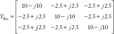
Since, the power system has three buses (n = 3), the size of YBus is 3 × 3. The elements of YBus by direct inspection as follows:
It can be verified that Y22 = Y33 = Y11.
Off-diagonal element Y12 = Y21 is:
It can be shown that,
The YBus of the power system network is
2.7.2 Step-by-Step Procedure
Now, we shall describe the step-by-step method for the case where there is no mutual coupling between the elements. The n × n sized YBus is initially set to zero. i.e., Yik = 0 for i = 1, 2, 3, …, n and k = 1, 2, 3, …, n. The elements are now added one at a time. The added elements may be between the reference node and bus (i), or between buses i and k.
Let the element with admittance y be added between the reference node (0) and the ith bus. In this case only the diagonal element will be affected.
Let the element with admittance y be added between the ith and kth buses.
In this case, four elements in the YBus, namely Yii, Yik, Yki and Ykk will be affected.

MATLAB Program for the step-by-step method and some numerical examples are presented below.
MATLAB PROGRAM FOR STEP-BY-STEP METHOD TO FORM YBus
% This Program Formulates YBus by step-by-step Method
% This Program is developed by Dr N.V. RAMANA
function ybus_direct
fprintf(‘ Enter “zdata” in this format at the MATLAB Prompt >> ’);
fprintf(‘ 1. From bus No. 2. To Bus No. ’);
fprintf(‘ 3. Element Resistance 4. Element Reactance ’);
fprintf(‘ As an example enter zdata at the command prompt in this way: ’);
fprintf(‘zdata = ’);
fprintf(‘[1 2 0 0.25; 1 3 0 0.12; 1 0 0 0.1; 2 0 0 0.2; 2 3 0 0.15; 3 0 0.05 0.15]; ’);
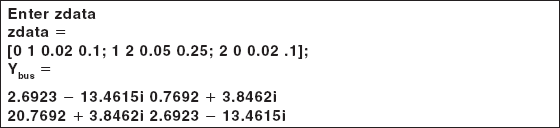
disp(‘enter zdata’);
zdata = input(‘zdata = ’);
nl = zdata(:,1); nr = zdata(:,2); R = zdata(:,3); X = zdata(:,4);
nbr = length(zdata(:,1)); nbus = max(max(nl), max(nr));
Z = R + j*X; %branch impedance
y = ones(nbr,1)./Z; %branch admittance
ybus = zeros(nbus,nbus); % initialize ybus to zero
for k = 1:nbr; % off diagonal elements formation
if nl(k) > 0 & nr(k) > 0
ybus(nl(k),nr(k)) = ybus(nl(k),nr(k)) 2 y(k);
ybus(nr(k),nl(k)) = ybus(nl(k),nr(k));
end
end
for n = 1:nbus % diagonal elements formation
for k = 1:nbr
if nl(k) == n | nr(k) == n
ybus(n,n) = ybus(n,n) + y(k);
else, end
end
end
ybus
Example 2.13
Using the data in Example 2.12, obtain YBus by step-by-step procedure.
Solution:
Step-1: Set all the elements in the [YBus]3 × 3 matrix as zeros.
Step-2: Add element G1 between the reference node (0) and bus (1). In this case, only Y11 will be affected.
Therefore Y11,new = Y11,old + yG1 = 0 + 5 – j5 = 5 – j5 p.u
Step-3: Add element L1 between buses 1 and 3. Four elements will be affected.
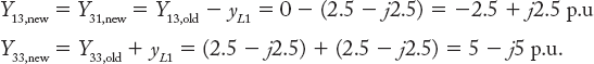
Step-4: Add element L2 between the buses 1 and 2. Four elements will be affected.
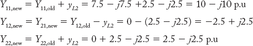
Step-5: Add element G2 from buses 0 and 2. Only Y22 will be affected:
Step-6: Add element L3 between buses 2 and 3. Four elements will be affected:
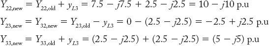
Step-7: Finally, add element G3 between the reference bus (0) and node 3. Only Y33 will be affected
Now by filling all elements, the YBus obtained by the step-by-step procedure is:

which is the same as that obtained by the direct inspection method.
Example 2.14
For the power system network shown in Figure 2.25, a new line L4 with an impedance of 0.25 1 j0.25 p.u is added between bus 1 and 2. Obtain the modified YBus.
Solution ![]()
The new line L4 is added between buses 1 and 2. Four elements of YBus will be affected.

Finally,
The modified YBus is:

Verification:
Due to addition of L4 between the buses 1 and 2, I1 and I2 are affected as:
Substituting the numerical values,
Solving,
From the above calculation, the modified YBus elements are:
2.8 Network Matrices by Singular Transformation Method
A few transmission lines in the power system may have mutual coupling. The easiest method for the formation of impedance/admittance network matrix is either the singular or the non-singular transformation method, in which the mutual effect can be easily included.
This section presents various network matrices obtained by the singular transformation method. First we start with the formation of the bus admittance matrix.
2.8.1 Bus Admittance Matrix
The performance equation in the admittance form is:
The relation between branch voltages and bus voltages can be written according to Equation 2.15 as:
where [v] is the (e × 1) column matrix of branch voltages,
[V] is (n × 1 × 1) the column matrix of bus voltages, and
A is the bus incidence matrix.
By substituting, Equation (2.15) in Equation (2.9),
Pre-multiplying both sides of the above equation by AT,
In Equation 2.16, AT I represents the sum of all currents meeting at the bus. Therefore according to KCL
Also, ATJ can be designated as IBus as it represents the algebraic sum of source currents or injected currents at each bus. Therefore Equation (2.16) modifies to:
from the above Eq. (2.17), the equation for YBus is:
where [Y] in the primitive admittance matrix.
Matlab Program for YBus formation by Singular Transformation Method.
% Student can use this program for forming YBus by Singular-Transformation Method
% This program is useful to form YBus, when the elements have mutual coupling
%This program is developed by Dr N.V.RAMANA
%-----------------------------------------------------------------------------------------
fprintf(‘Take reference bus 0 always ’)
elements = input(‘enter number of elements = ’);
zdata = zeros(elements,6);
fprintf(‘enter data in this format: 1.Element no. 2.From bus no. 3.To bus no. 4.Self impedance ’)
fprintf(‘ 5.Mutually coupled to element no 6. Mutual Impedance Value ’)
fprintf(‘ if element has no mutual coupling enter Item 6 as zero ’)
fprintf(‘when the program ask for “zdata”, enter like the following example: ’)
fprintf(‘Zdata = [1 0 2 0.25j 2 0.01j; 2 0 1 0.2j 1 0.01j; 3 1 3 0.25j 0 0;4 1 2 0.3j 0 0; 5 2 3 0.1j 0 0]; ’)
yprimitive = zeros(elements,elements);
zprimitive = zeros(elements,elements);
zdata = input(‘enter Zdata = ’);
%formation of primitive impedance matrix
x = zdata(:,5);
for i = 1:elements
zprimitive(i,i) = zdata(i,4);
if x(i)~ = 0
zprimitive(x(i),i) = zdata(i,6);
end
end
%formation of bus incidence matrix A begins
nb = max(max(zdata(:,2)),max(zdata(:,3)));
%initialize A matrix
nbuses = nb – 1;
A5zeros(elements,nbuses); % gives size of matrix A and is initialized to zero
for i = 1:1:elements,
if zdata(i,2)~ = 0 % formation of matrix A
A(i,zdata(i,2)) = 1;
end % end for ‘if’ statement
if zdata(i,3)~ = 0
A(i,zdata(i,3)) = – 1;
end % end for ‘if’ statement
end
yprimitive = inv(zprimitive);
ybus = A’*yprimitive*A
Example 2.15
Obtain primitive admittance matrix [Y] for a four element power system, elements 2 and 3 have mutual reactance of Xm and the self reactances of individual elements are Xsi for i = 1, 2, 3 and 4.
Solution:
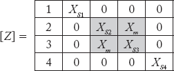
Now, the primitive admittance matrix [Y] can be obtained from [Y] = Z–1
Example 2.16
Obtain YBus by the singular transformation method for the power system shown in Figure 2.25, using the data in Example 2.12,
Solution:
The graph of the network in Figure 2.25 is shown below:
Here,
No. of elements e = 6; No. of nodes n = 4.
No. of branches b = 3 (elements 1, 2 and 3); No. of links l = 3 (elements 4, = and 6)

Fig 2.29 Graph of the Power System Network Shown in Figure 2.25
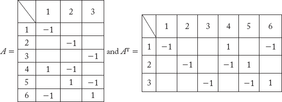
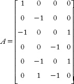
The matrix A can be written as
The primitive [Z] matrix can be written as:

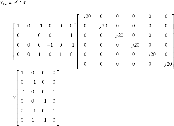
and primitive [Y] = Z–1

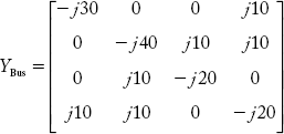
The multiplication of the two matrices [Y] and [A] yields

and
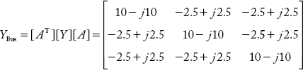
It can be verified that the YBus obtained by this method is same as that obtained by the earlier methods.
2.8.2 Branch Admittance Matrix
Consider the graph shown in Figure 2.12. In the graph elements 1, 2 and 3 are branch elements and 4, 5 and 6 are link elements. Let vb1, vb2, vb3, vl4, vl5, and vl6 be voltage drops across the branch and link elements.
The voltage drop across the elements in the matrix form is:
where vb is the branch voltage matrix VBr.

Following the orientation of the elements as the direction of current and with the application of KVL, the link voltages can be expressed in branch voltages as:

Therefore, element voltages in terms of branch voltage are:
Finally, the relation between voltage drop across all the elements in terms of branch voltage can be written as:

It can be proved that the coefficient matrix is the same as the fundamental cutset incidence matrix. Therefore the above equation can be written as:
Branch Admittance Matrix
The primitive network performance equation for a system with e number of elements can be written as:
where I the element current and J is the source current in parallel with the elements of dimension (e × 1) each.
[v] Matrix represents element voltages of size (e × 1).
Multiplying both sides of Equation (2.9) by CT, where C is the cutset incidence matrix.
CT [I] = 0, since the sum of all currents meeting at a node is zero,
The source current matrix [J] can be partitioned into:

where Jb is the source acting in parallel across the branches and it can be proved that
By substituting Equation (2.19) and (2.21) in Equation (2.20), it modifies to:
and from the above equation,
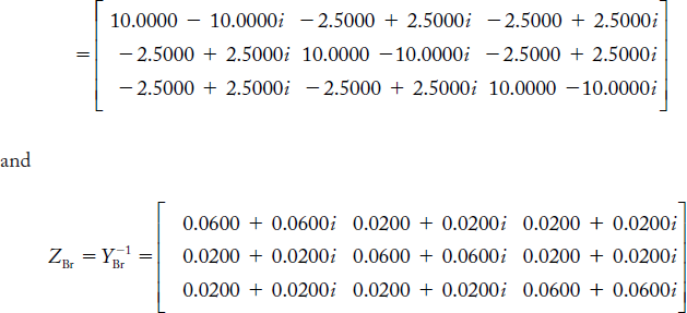
and ZBr = YBr–1 5 [CT [Y] C]–1
Example 2.17
Obtain YBr by singular transformation method for the power system shown in Figure 2.25, using the data in Example 2.12.
Solution:
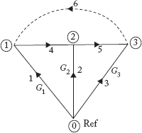
Fig 2.30 Graph of the Power System Network Shown in Figure 2.25
The f-cutset incidence matrix is

The primitive admittance matrix
and
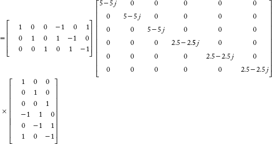
YBr = [CT][Y][C]
2.8.3 Loop Impedance Matrix or Admittance Matrix
To develop a loop impedance matrix or admittance matrix, we need to develop a relation between loop currents and branch currents. Remembering that whenever a link is added for the existing tree a new loop is created and that the loop currents are same as the link currents,
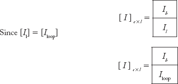
Iloop = [Il] of dimension (l × l)
The current matrix for all the elements can be partitioned as:
Now, we shall develop a relation between loop currents (or link currents) and branch currents Ib. It is easier to establish the relation with the help of an example. Consider the graph shown in Figure 2.31.
The following relations can be obtained based on the relation between link currents and loop currents:
Now, the branch currents are
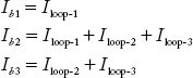
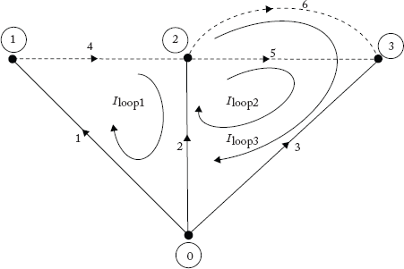
Fig 2.31 Graph Showing f-Loops and Open Loops of the Graph Shown in Figure 2.12
Now, the element current matrix [I] can be shown as
Comparison of the above coefficient matrix with the f-loop incidence matrix (L) obtained in Section 2.4.6 shows that both are the same.
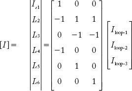
Hence, the element current matrix [I] can be written in terms of L and [Iloop] matrix as:
Loop Impedance Matrix
Consider the primitive network performance equation in the impedance form
Multiplying both sides of Equation (2.7) by LT
LT [v] represents the algebraic sum of voltages in a closed loop. Its value is zero according to Kirchoff's voltage law. Similarly, LT [e] gives the sum of algebraic sum of source voltages around each basic loop.
Therefore,
Substituting (2.26) and (2.24) in Equation (2.25)
From the above equation
and
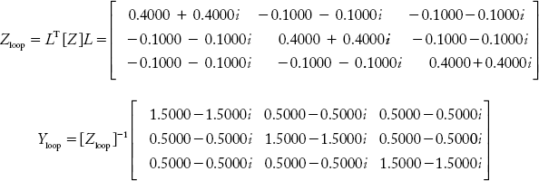
Example 2.18
Obtain Zloop and Yloop matrices by singular transformation methods for the power system shown in Figure 2.25. Use the data given in Example 2.12.
Solution:
Refer Section 2.4.6, for the f-loop incidence matrix:

The primitive impedance matrix [Z] is

2.9 Network Matrices by Non-Singular Transformation Method
This transformation method uses augmented incidence matrices, which are square and non-singular matrices. The primitive impedance [Z] or admittance [Y] matrices are transformed into network matrices by using these augmented incidence matrices.
2.9.1 Branch Admittance Matrix
Consider the augmented cutset incidence matrix Ĉ in the partitioned form.

In order to form tie-cutsets, we shall modify the existing network by introducing a fictitious branch in series with each link element in the augmented primitive network as shown in Figure 2.29.

Fig 2.32 Augmented Primitive Network
Due to these fictitious changes in the network, the performance of the network should not be affected. For this purpose, the following assumptions are made:
- The admittance of each fictitious branch is equal to zero. Through this assumption, the voltage across each branch is zero.
- Current source Jik across the fictitious branch is set to be equal to the current through the associated link (i.e JL = Jik = Iik).
Now, the performance equation for the augmented network in the branch frame of reference is:
In Equation (2.30), ÎBr, ![]() Br are column matrices of dimension (e × 1) and ŶBr is a square matrix of size (e × e).
Br are column matrices of dimension (e × 1) and ŶBr is a square matrix of size (e × e).
From Equation (2.9), the performance equation for the primitive network is:
Multiplying (2.9) by Ĉ T,
Equation (2.31) can be rewritten by including sub-matrices of ĈT, element current [I] and source current [J] matrices.
[v] represents element voltages.
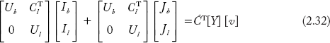
In Equation (2.32), the matrices I and J are partitioned with respect to branches and links as:
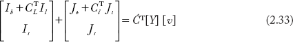
On the left hand side of Equation (2.33), it can be proved that,
Following the discussion in Section (2.9.2)
Then the left hand side of Equation (2.32) can be written as:
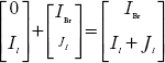
Now, Equation (2.33) modifies to:

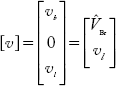
Hence, we may write the modified element voltage matrix [v] for the augmented network as:

In the portioned matrix Equation (2.35), vf elements are the voltages of fictitious branches which are set to zero.
The augmented branch voltage matrix ![]() Br can be written as:
Br can be written as:

Repeat Equation (2.19)
The element voltage matrix v, for the original network can be written as:
and for the augmented network it is:
Multiplying Equation (2.36) by Ĉ
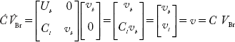
From the above,
Use of the above relation in Equation (2.34) gives
From Equation (2.38), the augmented branch admittance matrix can be written as:
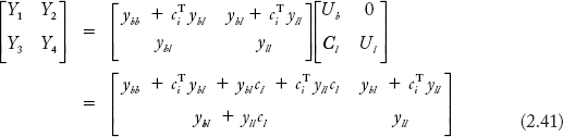
The augmented admittance matrix in Equation (2.39) can be written in the partitioned form as:

In Equation (2.40), the primitive admittance matrix [Y] is written in the partitioned form as shown below:
Multiplying the matrices on the right hand side of Equation (2.40) yields:
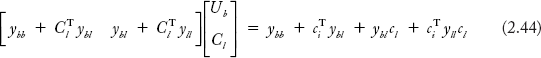
Extracting Y1 from the above equation yields:
The equation for Y1 can be shown to be the same as that obtained from Equation (2.23) as:
Expanding the RHS of Equation (2.23),

Multiplying the matrices in Equation (2.43),
Thus, the equation for Y1 in Equation (2.42) and YBr in Equation (2.44) are verified to be the same Therefore, the branch admittance matrix through non-singular transformation method is:

2.9.2 Loop Impedance and Loop Admittance Matrix
Zloop or Yloop can be obtained using the augmented loop incidence matrix ![]() by the non-singular transformation method. By adding fictitious open loops equal to the number of branches, the L matrix is augmented into a square
by the non-singular transformation method. By adding fictitious open loops equal to the number of branches, the L matrix is augmented into a square ![]() matrix. However, the changes in the
matrix. However, the changes in the ![]() , should be in accordance with the changes in the primitive network. In an augmented network, a fictitious link is added in parallel with every branch element of the network. This introduces a fictitious loop containing the branch and the fictitious link. However, these changes should not affect the performance of the network. For this purpose the following assumptions are made:
, should be in accordance with the changes in the primitive network. In an augmented network, a fictitious link is added in parallel with every branch element of the network. This introduces a fictitious loop containing the branch and the fictitious link. However, these changes should not affect the performance of the network. For this purpose the following assumptions are made:
- The impedance of each fictitious link is zero.
- A voltage source is connected in series with the fictitious link. It is then set equal and opposite to the voltage across the associated element such that, current flowing through the fictitious link is zero. This will not affect the branch current. Addition of the fictitious link creates an ‘open loop’ since no current flows inside the loop.
For example, consider an open loop of a branch connected between reference node 0 and node 2 as shown in Figure 2.33.
The performance equation of the augmented network in the loop frame of reference is:
where Ẑloop is the augmented network loop impedance matrix.
The performance equation of a primitive network in impedance form is

Fig 2.33 Introducing an Open Loop by Addition of a Fictitious Link
Multiplying both sides by [![]() ]T,
]T,
Equation (2.47) in the partitioned form can be written as:

In Equation (2.48), the voltage across element matrix [v], and series source voltage matrix [e] are partitioned with respect to branches and links.
Multiplying matrices in Equation (2.48),

It can be proved that
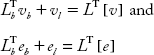
As the algebraic sum of voltages in a closed loop is equal to zero:

Therefore Equation (2.49) is modified as:
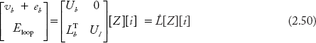
In Equation (2.50), vb + eb represents the algebraic sum of voltages in open loops. The augmented loop voltage matrix Êloop is:

Similarly, the augmented loop current matrix can be partitioned as

Since the open loop currents ib are set to zero above equation modifies to:
The currents through all the elements of the original network is given by
It can be proved that,
From (2.53) and (2.54)
Substituting Equation (2.55) in (2.51), the latter modifies to:
From Equation (2.56), the augmented loop impedance matrix Ẑloop is:
Equation (2.57) is partitioned as:
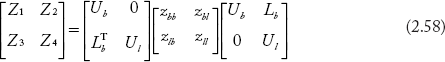
By extracting Z4 from Equation (2.58) and comparing it with Equation (2.28), the equation for Zloop can be obtained as:
And
2.9.3 Bus Admittance and Bus Impedance Matrices
Both A and  matrices are not square matrices and hence cannot be used in the non-singular transformation method to obtain YBus. However, Yloop, YBr, Zloop, and ZBr, matrices can be obtained by the non-singular transformation method. The following methods describe the method of obtaining YBus or ZBus through branch- and loop-network matrices.
Method-1: YBus and ZBus from ZBr,
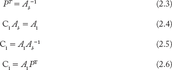
Repeat Equations from (2.2) − (2.6) for convenience
The matrix A can be partitioned as

Post-multiply with A by PT
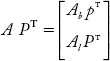
Substituting Equations (2.2) and (2.6) in the above equation,

Transpose the above equation
Post-multiply Equation (2.62) by [y] APT,
The above equation is rewritten as
From the above
and
Substituting PT = Ab−1 (Equation 2.3) in the above equation
Using Equation (2.63) YBus may be represented as:
Using Equation (2.3) in (2.65), Equation (2.65) modifies to
and as
Therefore
Method-2: YBus and ZBus from Zloop
The augmented loop impedance matrix is given by
Ẑloop =  where Z1, Z2, Z3 and Z4 are partitioned matrices as discussed earlier and the loop admittance matrix is:
It can be shown that,
as,

Multiplication of the matrices in Equation (2.68) yields.

From the third equation in (2.69),
Substituting Z3 in the last equation in (2.69)
Rewrite the above equation as
It was obtained earlier that
Also,
Based on the above equation and Equation (2.70), the equation for Yloop can be obtained as:
The first and third equations in (2.69) are repeated.
From the second equation of the above,
Substituting Y3 in the first equation of the above,

From Equation (2.45)
Substituting (2.45) in (2.72), we can obtain ZBr as
Now, ZBus can be obtained by using Equation (2.67) as
2.9.4 Algorithm for Singular and Non-Singular Transformation Methods
Step-A: To obtain the network impedance/admittance matrix, the primitive impedance matrix [z] is first developed.
- [z] is a diagonal matrix, if elements have no mutual coupling.
- Mutual impedances can be entered as off-diagonal elements in the [z] matrix.
- After obtaining [z], the primitive admittance matrix [y] can be obtained as:
It may be recollected that if elements have no mutual coupling then, the diagonal elements of [y] can be obtained directly by taking the reciprocal of the diagonal elements of [z].
Step-B: For the singular transformation method, go to Step C; and for the non-singular transformation method, go to Step-D.
Step-C: Network matrices by the singular transformation method:
The following formulae can be used
| YBus or ZBus | YBr or ZBr | Yloop or Zloop |
|---|---|---|
| 1. Convert the network into a graph and obtain the bus incidence matrix [A]. 2. Obtain YBus as YBus = AT[y]A 3. Obtain ZBus as ZBus = Y-1Bus |
1. Convert the network into a graph and obtain the basic or f-cutset incidence matrix [C]. 2. Then obtain YBr as YBr = CT[y]C. 3. Obtain ZBr as ZBr = YBr-1 |
1. Convert the network into a graph and obtain the basic or f-loop incidence matrix [L]. 2. Then obtain Zloop as Zloop = LT[z]L 3. Obtain Yloop as Yloop = Z-1loop. |
RETURN
Step-D: Network matrices by non-singular transformation method
Step-1: Convert the network into a graph and obtain the augmented loop incidence matrix (![]() )
)
Step-2: Partition ![]() into
into

In the matrix ![]() ,
,
Ub: Identity matrix corresponding to open loops (branches) of dimension (b × b)
Lb: Partitioned sub-matrix corresponding to basic or f-loops of dimension (b × l).
O: Null matrix of dimension (l × b)
Ul: Identity matrix corresponding to f-loops of dimension (l × l).
(b: no. of branches, l: no. of links)
Step 3: Obtain the augmented loop incidence matrix as Ẑloop = [![]() ]T[z][
]T[z][![]() ]
]
where the z-matrix is obtained initially.
Step-4: Partition Ẑloop into:

The partitioned matrices Z1, Z2, Z3, Z4 have the following dimensions:
Step-5: If Zloop or Yloop is required, go to Step-6. If ZBr, YBr, or ZBus is required, go to Step-7.
Step-6: Zloop = Z4 and Yloop = [Z4]-1
RETURN
Step-7: Calculate ZBr by using the following formula.
and YBr = ZBr-1
Step-8: If ZBus or YBus is required go to Step-9, otherwise print
ZBr or YBr and
RETURN
Step-9: ZBus and or YBus can be determined by using following formulae:
Formula-1 : YBus = AbT YBr Ab
ZBus = YBus-1 (To use this formula the bus incidence matrix A is required.)

Formula-2: Use ZBus = [PT][ZBr][P]
where P is the branch path incidence matrix and
RETURN
END
Example 2.19
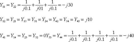
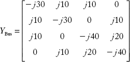
Figure 2.34 represents an oriented graph of a power system network. The element numbers are marked in the figure. The reactances in per unit are given below:
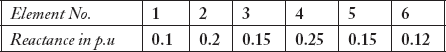
Formulate YBus by:
- Direct inspection method
- Singular transformation method
- Non-singular transformation method

Fig 2.34 Oriented Graph for the Network in Example 2.10
Solution:
(a) Direct inspection method:

The above elements are entered in a bus admittance matrix as given below:
The student can run MATLAB Program ybus_direct and verify the result obtained.
MATLAB RESULT
>> ybus_direct
Enter “zdata” in this format at the MATLAB Prompt >>
1. From Bus No. 2. To Bus No.
3. Element Resistance 4. Element Reactance
As an example enter zdata at the command prompt in this way:
zdata =
[1 2 0 0.25; 1 3 0 0.12; 1 0 0 0.1; 2 0 0 0.2; 2 3 0 0.15; 3 0 0.05 0.15];
Enter zdata
zdata =
[1 2 0 0.25; 1 3 0 0.12; 1 0 0 0.1; 2 0 0 0.2; 2 3 0 0.15; 3 0 0 0.15];
ybus =
0 − 22.3333i 0 + 4.0000i 0 + 8.3333i
0 + 4.0000i 0 − 15.6667i 0 + 6.6667i
0 + 8.3333i 0 + 6.6667i 0 + 221.6667i
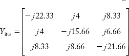
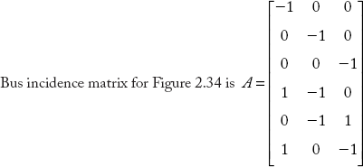
(b) Singular transformation method:
For the oriented graph in Figure 2.34 the A and Y matrices are
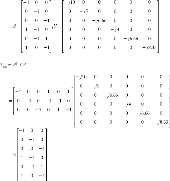
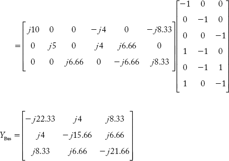
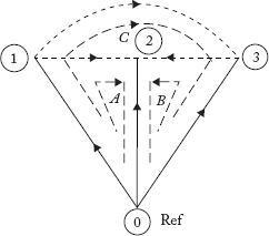
Fig 2.35(a) Graph Showing f-Loops
(c) Non-singular transformation method:
For an oriented graph the augmented loop incidence matrix
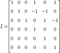
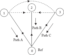
Fig 2.35(b) Graph Showing Paths
Primitive impedance matrix is
Branch path incidence matrix, P for the oriented graph in Figure 2.5(b), may be given as below:
The student can run MATLAB program YBus_singular for YBus and verify the result.
MATLAB RESULT
>> ybus_singular
Always take Reference Bus as 0
Enter number of elements = 6
Enter data in this format: 1.Element No. 2.From Bus No. 3.To Bus No.
4.Self-impedance 5.Mutually coupled to Element No. 6. Mutual Impedance Value
If the element has no mutual coupling enter Item 6 as zero
When the program asks for “zdata”, enter as given in the following example:
Zdata = [1 0 2 0.25j 2 0.01j; 2 0 1 0.2j 1 0.01j; 3 1 3 0.25j 0 0; 4 1 2 0.3j 0 0; 5 2 3 0.1j 0 0];
Enter zdata =
[1 2 0 0.25; 1 3 0 0.12; 1 0 0 0.1; 2 0 0 0.2; 2 3 0 0.15; 3 0 0 0.15];
ybus =
0 − 22.3333i 0 + 4.0000i 0 + 8.3333i
0 + 4.0000i 0 − 15.6667i 0 + 6.6667i
0 + 8.3333i 0 + 6.6667i 0 + −21.6667i
Example 2.20
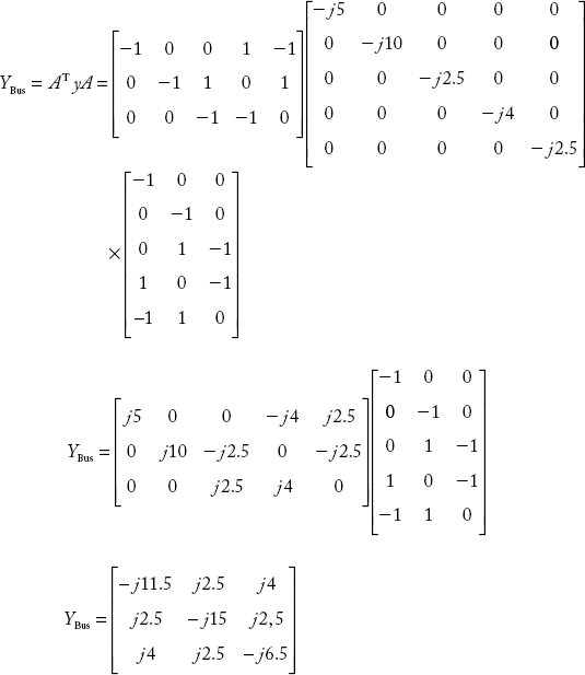
Form the YBus by using singular transformation for the network shown in Figure 2.36(a)

Fig 2.36(a) Network for Example 2.20
Solution:
Primitive admittance matrix Y is given by:
Bus incidence matrix from Figure 2.36 (a) is:

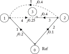
Fig 2.36(b) Network for Example 2.20
By singular transformation method,
The student can run MATLAB program ybus_singular for ybus and verify the result.
MATLAB RESULT
enter Zdata 5 [1 1 2 0.4j 0 0; 2 1 3 0.25j 0 0; 3 1 0 0.2j 0 0; 4 2 0 0.1j 0 0; 5 2 3 0.4j 0 0];
ybus =
0 − 11.5000i 0 + 2.5000i 0 + 4.0000i
0 + 2.5000i 0 − 15.0000i 0 + 2.5000i
0 + 4.0000i 0 + 2.5000i 0 − 6.5000i
Example 2.21
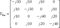
Figure 2.37 indicates the graph of a power system network. The p.u reactance of each element is taken as j0.1p.u. Formulate YBus by the singular transformation method and verify the same with the YBus obtained by the direct inspection method.
Solution:
A) Singular transformation method:
Bus incidence matrix for the given graph is:


Fig 2.37 Graph of the Power System Discussed in Example 2.21
Primitive admittance matrix Y elements are given below:
Diagonal elements of [y]
and off-diagonal elements are zero.
YBus = AT y A
The student can run MATLAB program ybus_singular for ybus and verify the result.
MATLAB RESULT
Enter Zdata = [1 1 2 0.1j 0 0; 2 1 3 0.1j 0 0; 3 1 0 0.1j 0 0; 4 2 0 0.1j 0 0; 5 2 4 0.1j 0 0; 6 3 0 0.1j 0 0; 7 3 4 0.1j 0 0; 8 3 4 0.1j 0 0; 9 4 0 0.1j 0 0];
ybus 5
0 = 30.0000i 0 + 10.0000i 0 + 10.0000i 0
0 + 10.0000i 0 − 30.0000i 0 0 + 10.0000i
0 + 10.0000i 0 0 − 40.0000i 0 + 20.0000i
0 0 + 10.0000i 0 + 20.0000i 0 − 40.0000i
B) Direct inspection method:
The matrix formed by entering all the elements of the YBus, is given below:
Example 2.22
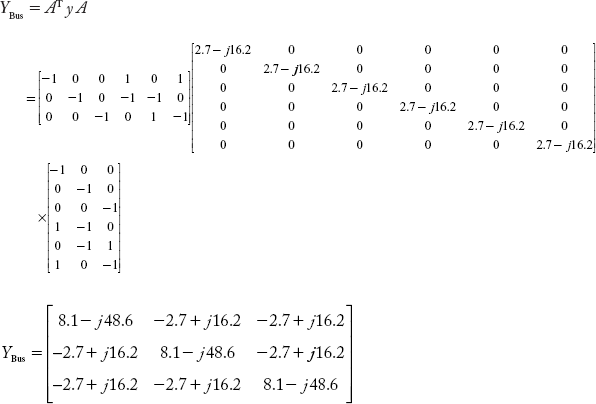
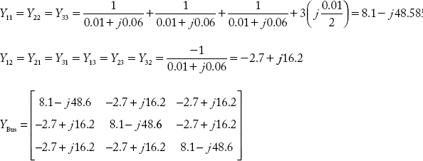
Consider the linear graph in Figure 2.38 of a power system. Each element has a series impedance of (0.01 1 0.06) p.u. Compute YBus by singular transformation and verify the result with that obtained by the direct inspection method.
Solution:
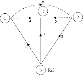
Fig 2.38 Oriented Graph for the Power System in Example 2.22
Singular transformation method
Primitive admittance matrix elements are:
The student can run the MATLAB program YBus_singular for YBus and verify the result.
MATLAB RESULT
Enter Zdata = [1 1 2 0.01 + 0.06j 0 0; 2 1 3 0.01 + 0.06j 0 0; 3 1 0 0.01 + 0.06j 0 0; 4 2 0 0.01 + 0.06j 0 0; = 2 3 0.01 + 0.06j 0 0; 6 3 0 0.01 + 0.06j 0 0];
YBus =
8.1081 − 48.6486i − 2.7027 + 16.2162i − 2.7027 + 16.2162i
−2.7027 + 16.2162i 8.1081 − 48.6486i − 2.7027 + 16.2162i
−2.7027 + 16.2162i − 2.7027 + 16.2162i 8.1081 − 48.6486i
Verification of answer by direct inspection method
Example 2.23
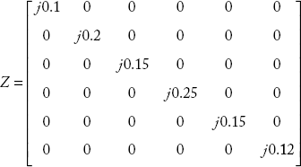
Figure 2.39(a) shows a six-element graph of a power system network. Each element reactance is j0.1 p.u. Formulate ZBus, Zloop, ZBr and YBus by the non-singular transformation method. Verify the YBus using the direct inspection method.
Solution:
Non-singular transformation method:
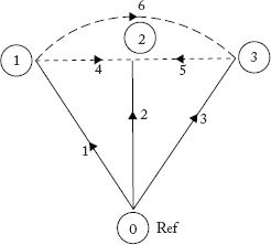
Fig 2.39(a) Oriented Graph of the Power System in Example 2.23
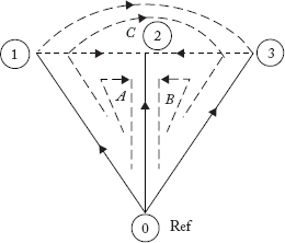
Fig 2.39(b) f-Loops Graph for Example 2.23
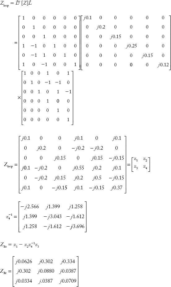
From the oriented graph, the augmented loop incidence matrix and the primitive impedance matrix are given as

The equation for Zloop is:
Each of the sub-matrices in Zloop is of the order 3 × 3.
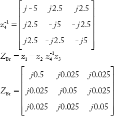

Fig 2.39(c) Paths of the Graph for Example 2.23
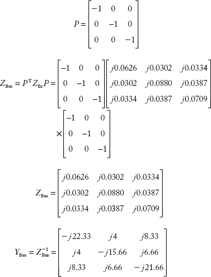
Branch path incidence matrix, P for Figure 2.39(c) is:

Direct inspection method:
Substituting the above elements the value of YBus can be obtained as:
The student can run MATLAB program YBus_singular for YBus and verify the result.
MATLAB RESULT
Enter zdata
zdata =
[1 2 0 0.1; 1 3 0 0.1; 1 0 0 0.1; 2 0 0 0.1; 2 3 0 0.1; 3 0 0 0.1];
Ybus =
0 − 30.0000i 0 + 10.0000i 0 + 10.0000i
0 + 10.0000i 0 − 30.0000i 0 + 10.0000i
0 + 10.0000i 0 + 10.0000i 0 − 28.0000i
Example 2.24
For the power system transmission network shown in Figure 2.40(a), formulate YBus by the singular transformation method. The self and mutual reactances in p.u are indicated in the figure. Take Bus (1) as reference.

Fig 2.40(a) Power System for Example 2.24
Solution:
Singular transformation method:
Primitive admittance matrix Y is obtained from Z as:


Fig 2.40(b) Graph of the Power System for Example 2.24

The student can run MATLAB program YBus_singular for YBus and verify the result.
MATLAB RESULT
Enter Zdata 5 [1 0 1 0.20j 4 0.01j; 2 1 2 0.3j 0 0; 3 0 3 0.25j 0 0; 4 0 1 0.3j 1 0.01j; 5 2 3 0.35j 0 0];
Ybus =
0 − 11.3467i 0 + 3.3333i 0
0 + 3.3333i 0 − 6.1905i 0 + 2.8571i
0 0 + 2.8571i 0 − 6.8571i
Example 2.25
Figure 2.41(a) shows a 3-Bus power system transmission network. The line impedances are given below:

Formulate YBus for the following cases:
- Assume that the line shown dotted between Bus 2 and Bus 3, that is line 2–3(2) is not present.
- Discuss which elements of YBus obtained in Case-(a) are effected when the dotted line 2–3(2) is connected. The new line has no mutual coupling with other lines.
- Obtain the modified YBus when line 2–3(2) which has mutual impedance of (0 + j0.01) p.u. when line 223(1) is connected.
Fig 2.41(a) Power System for Example 2.25
Fig 2.41(b) Graph for Example 2.25
Solution:
(a) Direct inspection method:

The student can run MATLAB program YBus–direct for YBus and verify the result.
(b) A new line is connected between Bus 2 and Bus 3.
Singular transformation method:
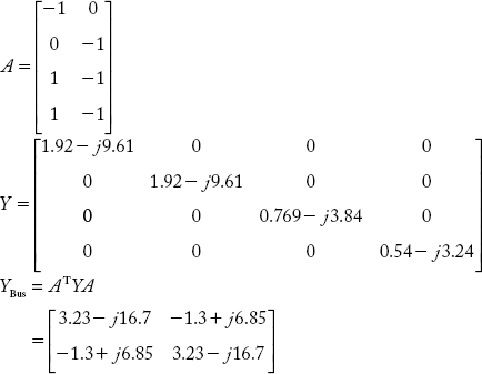

Fig 2.41(c) Addition of Line Between Buses 2 and 3
The student can run MATLAB program YBus–singular for YBus and verify the result

Because of newly connected line between Bus 2 and Bus 3, the elements connected to these two buses are affected.
Therefore y22, y33, y23, y32 are changed.
(c) The newly connected line between Bus 2 and Bus 3 has a mutual coupling with the already existing line.
Fig 2.41(d) Graph with Mutual Coupling
Singular transformation method
Primitive impedance matrix

Because of the addition of a line and mutual coupling between lines 3 and 4 the primitive admittance matrix (y) and YBus has changed.
Example 2.26
For the power system network shown in Figure 2.42(a) obtain YBus by the singular transformation method. The reactance of each line is 0.01 p.u and that of the generator is j0.05 p.u. Each line has a half-line charging admittance of j0.05 p.u.
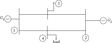
Fig 2.42(a) Power System Network for Example 2.26
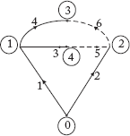
Fig 2.42(b) Graph for the Network Shown in Figure 2.42(a)
Solution:
We use the singular transformation method to solve this problem. The oriented graph for Figure 2.42(a) is given in Figure 2.42(b). Bus incidence matrix A is:
Primitive admittance matrix is:

Note:
The student is advised to solve the above problem by using the presented MATLAB programs and verify the same.
Questions from Previous Question Papers
1. Define the following by taking a suitable graph as example:
Graph, Sub-Graph, Tree, Co-Tree, Path, Loops and Cutsets.
2. For the power system shown in Figure Q1, obtain the following:
(a) Oriented Graph, (b) Tree, (c) f-Cutsets, (d) f-Loops

Fig Q1
3. For the network shown in Figure Q2 obtain all incidence matrices.
4. Explain about augmented incidence matrices.
5. Explain primitive network and primitive network matrices.
6. Develop primitive impedance and admittance matrices for the network shown in Figure Q2.2.
7. Deduce the relation YBus = AT[Y]A
8. All the elements in Figure Q2.2 have equal reactances of j0.1 p.u. each. Obtain all the YBus by singular transformation method and verify the same using the direct inspection method.
9. Obtain ZBr, Zloop and YBus by the non-singular transformation method
10. The transpose of a bus incidence matrix of a transmission network is:
Draw the oriented graph of the network.
11. Define the following terms with suitable examples
- Tree
- Branches
- Links
- Co-tree (v) Loop
12. Explain the following terms
- Basic Loops
- Cut-set
- Basic cut sets
- Loop
By taking an oriented connected graph, show the relation between basic loops, links and basic cut sets and the number of basic cut-sets and number of branches.
13. What is the relation among the number of nodes, number of branches, number of links and number of elements?
14. For the power system network shown in Figure Q2 below, draw the
- Oriented graph
- Tree and co-tree of the corresponding graph, also show the basic loops and basic cutsets for the same.
Fig Q2
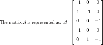
15. The incidence matrix for an oriented graph is given below. Draw the oriented graph.
16. What is the bus-incidence Matrix A? and what is the dimensions of this matrix?
17. For the graph shown in Figure Q3 write down the A and ![]() matrices. (Take 1-2-3-4 as tree elements)
matrices. (Take 1-2-3-4 as tree elements)
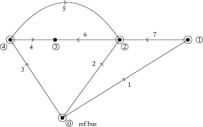
Fig Q3
18. The rows of the bus incidence matrix A are arranged according to a particular tree and the matrix A is partitioned into submatrices Ab of dimension (b × (n-1)) and Al of dimensions (l × (n × 1)). where the rows of Ab correspond to branches and rows of Al correspond to links. Show the above partitions for the matrix A for the simple network shown in Figure Q4. Also, form the element node incidence matrix ![]()

Fig Q4
19. For the oriented connected graph in Figure Q6 obtain the bus incidence matrix, branch-path incidence matrix and basic cut-set matrix.

Fig Q6
20. For the sample network shown in Figure Q7, form (a) The incidence matrices ![]() , A, P, C,
, A, P, C, ![]() , L and
, L and ![]() and verify the following
and verify the following
- AbPT = U
- Cl = AlPT
- LBt – U
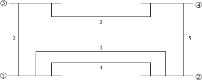
Fig Q7
Take node 1 as reference and elements 1, 2, 5 as tree branches.
21. Explain about augmented cut-set incidence matrix ![]() . What are the entries of the matrix.
. What are the entries of the matrix.
22. What does basic cut set incidence matrix C (obtained from an oriented connected graph) represents? What are the entries of this matrix and how are they determined?
23. For the graph given in Figure Q8, draw the tree and the corresponding co-tree. Choose a tree of your choice and hence write the cut-set schedule.

Fig Q8
24. For the network given in Figure Q9 draw the graph and tree. Write the cut-set schedule for a choosen tree branch set.
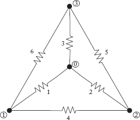
Fig Q9
25. For Figure Q10, develop basic cutset incidence matrix

26. What does basic loop incidence matrix L represent? What are the entries of this matrix and how are they determined?
27. Explain briefly about augmented loop incidence matrix ![]() .
.
28. Derive an expression for ZLoop for the oriented graph shown in Fig Q11.

29. For the graph shown in Figure Q12 selecting tree elements (2, 4, 5 and 6),
- Write the fundamental loop incidence matrix and the fundamental cutset matrix C. Verify the relation LCT = 0 and Lb = -ClT
- (b) Write the augmented incidence matrix and incidence matrix A by choosing (4) as reference node. Arranging matrix A as (Ab/Al) corresponding to the tree T elements (2, 4, 5 and 6) and verify Cl = AlAbT
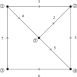
Fig Q12
30. What do you understand by branch-path incidence matrix P? What are the elements of matrix P and what is the nature of this matrix? What is the relationship between the branch-path incidence matrix P and the submatrix Ab of the bus incidence matrix A (Ab is of dimensions b × (m – 1))?
31. Taking node O as the reference, write down the branch-path incidence matrix P for Figure Q13 (take 1-2-3-5 as tree elements)
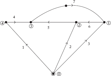
Fig Q13
32. For the network shown in Figure Q14, draw the graph and mark a tree. How many trees this graph can have? Mark the basic and form the bus incidence matrix A, the branch path incidence matrix P and also the basic loop incidence matrix.
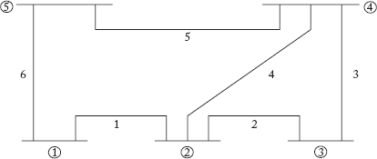
Fig Q14
33. For the network shown in Figure Q15, draw its graph and also mark a tree. Give the total number of edges (i.e. elements), nodes, buses and branches for this graph. Determine YBus matrix directly by inspection.

Fig Q15
34. Derive the expressions for bus admittance and impedance matrices by singular transformation.
35. Derive the expressions for the ZLoop using singular transformation in terms of primitive impedance matrix Z and basic loop incidence matrix L.
Competitive Examination Questions
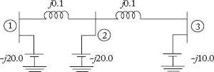
1. A sample power system network is shown in the figure below. The reactances marked are in p.u. The per unit value of Y22 of the bus admittance matrix (YBus) is

- j10.0
- j0.4
- –j0.1
- –j20.0
[GATE 1991, Q. No: 1.8]
2. The single-line diagram of a network is shown in the figure below. The line series reactance is 0.001 p.u/km and shunt syseptance is 0.0016 p.u/km. Assemble the YBus.
[GATE 1994, Q. No: 17]
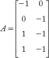
3. The network shown in the figure below has impedance in p.u as indicated. The diagonal elements Y22 of the bus admittance matrix YBus of the network is
[GATE 2005, Q. No: 60]
4. The figure below shows a dc resistive network and its graph is drawn aside. A proper tree chosen for analyzing the network will contain the edges.
- aa, bc, ad
- ab, ac, ca
- ab, bd, cd
- ac, bd, ad

[GATE 1994 Q. No: 1]
5. A connected network of N > 2 nodes has almost one branch directly connecting any pair of nodes. The graph of the network
- must have at least N branches for one or more closed paths to exist
- can have unlimited number of branches.
- can only have at most N branches.
- can have a minimum number of branches not decided by N.
[GATE 2001 Q. No: 2.2]
6. The graph of an electrical network has N nodes and B branches. The number of links, L, with respect to the choice of a tree is given by
- B – N + 1
- B + N
- N – B + 1
- N – 2B – 1
[GATE 2002 Q. No: 1.3]
7. If the number of branches in a network is B, the number of nodes is N, and the number of dependent loops is L, then the number of independent node equations will be
- N + L – 1
- B – 1
- B – N
- N – 1
[IES 2000 Q. No: 71]
8. An electric circuit with 10 branches and 7 nodes will have
- 3 loop equations
- 4 loop equations
- 7 loop equations
- 10 loop equations
[IES 2001 Q. No: 65]
9. The bus admittance matrix of the network shown in the figure below, for which the marked parameters are p.u impedances, is


[IES 1995 Q. No: 34]
10. The YBus matrix of a 100-bus interconnected system is 90% sparse, Hence the number of transmission lines in the system must be
- 450
- 500
- 900
- 1000
[IES 2002 Q. No: 103]
11. In the network shown, the marked parameters are p.u impedances. The bus admittance matrix of the network is
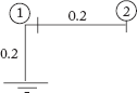


[IES 2003 Q. No: 39]
12. A sample power system network is shown in figure. The reactances marked are in p.u. The p.u value of Y22 of the Bus Admittance Matrix (YBUS) is:
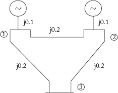
- j 10.0
- j 0.4
- –j 0.1
- –j 20.0
[GATE 1991 Q.No. 2]
13. The single line diagram of a network is shown in figure. The line series reactance is 0.001 p.u. per km and shunt susceptance is 0.0016 p.u. per km. Assemble the bus admittance matrix (YBUS) of the network, neglecting the line resistance.
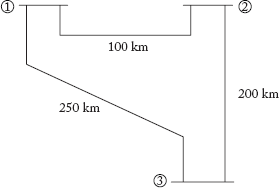
[GATE 1994 Q.No. 7]
14. For the given network in figure, obtain the bus admittance matrix (YBUS) using the data given:
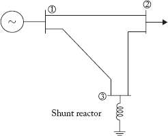
| Lines between nodes | Impedance p.u. | Half of line charging admittance |
| 1 – 2 | 0.0 + j 0.05 | j 1.25 |
| 1 – 3 | 0.0 + j 0.02 | j 0.50 |
| 2 – 3 | 0.0 + j 0.02 | j 0.50 |
| Shunt reactor at node | Impedance | |
| 1 – 2 | 0.0 + j 2.0 |
[GATE 1998 Q.No. 10]
15. The network shown in figure has impedances in p.u. as indicated. The diagonal element Y22 of the bus admittance matrix YBus of the network is:
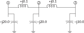
(a) –j 19.8
(b) +j 20.0
(c) +j 0.2
(d) –j 19.95
[GATE 2005 Q.No. 7]