CHAPTER 1

Introduction

1.1 Power System Studies

Power system network is the biggest man-made system in the world. This network is vast and it is difficult to understand its behaviour. A number of studies need to be conducted on the system for its operation and control. A ‘study’ is nothing but obtaining the values of system parameters. A system parameter, for example voltage or current, describes the condition of the system. A system parameter can be said to be either independent or dependent. An independent parameter varies on its own, while a dependent parameter is a function of an independent parameter. A system may be under two states, namely, steady state and dynamic or transient state and various studies may be conducted on the system when it is in either of these two states.

In the steady state of the system, system parameters are described as time invariant, while in the dynamic state, they vary with time. When a power system is in operation, it frequently switches over from one state to another. Therefore, the system condition needs to be analysed under both the states for better operation and control. Accordingly, some studies are categorised as steady state and others as dynamic state studies.

Any study can be unfolded into three stages:

Stage 1: Network modelling

Stage 2: Mathematical modelling

Stage 3: Solution

These stages are explained in the following sections.

1.1.1 Network Modelling Stage

A power system has three components: (1) generators, (2) transformers and (3) transmission lines. In this stage, we deal with how these components, along with their associated control equipment, can be represented as an equivalent electrical circuit component. The representation of equipment varies from one study to another. For example, an alternator is represented as a constant voltage source behind the reactance in stability and short-circuit studies, whereas the same alternator is represented as a complex power source in power flow studies. After representing each equipment by its appropriate circuit component model, a power system is converted into an electrical network.

1.1.2 Mathematical Modelling Stage

With the help of KCL and KVL, the network model is converted into a mathematical model. A mathematical model comprises of a set of mathematical expressions, describing the dependency of dependent system parameters on independent system parameters with a suitable function, either algebraic or differential. The type of mathematical model depends upon the type of study. For example, linear or non-linear algebraic equations are developed in steady state studies, while a set of linear or non-linear differential equations are developed in dynamical studies.

1.1.3 Solution Stage

Once an appropriate mathematical model is ready, we enter into the last stage of this study.

If the study has algebraic equations, we may use numerical methods like the Gauss–Seidel or the Newton–Raphson method. On the other hand, if the study has differential equations, then we may use methods such as the Runge–Kutta or Euler's method to solve them. The solution of the mathematical expressions gives the parametric values of dependent parameters for the known independent parameters. Once the parametric values of all system parameters are available, we may analyse the condition of the system, such as whether it is stable or unstable, controllable or uncontrollable, and so on.

We discuss power system studies under the following heads in this text book:

1. Power flow studies
2. Short-circuit studies
3. Stability studies

1.2 Organisation of Text Book

Apart from this chapter, this text book contains eight chapters.

Chapters 2 and 3 present the procedure of forming power system network matrices. Most of the system parameters and transmission line impedances can be conveniently represented in the matrix form. Power system network matrices describe the electrical properties of different components of the power system network. These chapters provide algorithms for the formation of network matrices and modifications required in the matrices to reflect changes in the network. MATLAB-based programs and solved numerical problems are also included.

Chapters 4 and 5 present an important power flow study. The study computes power flows in the transmission network for specified conditions at the buses. It is performed under steady state of the system and provide the initial state of the system required for all types of dynamical studies. The study has paramount importance in power system planning, operation and control. A mathematical model of the study comprises of a set of non-linear simultaneous algebraic equations. These equations can be solved by using either the Gauss–Seidel or the Newton–Raphson method. Chapters 4 and 5, respectively, deal with these methods.

Balanced and unbalanced fault analyses are included in Chapters 6 and 7, respectively. Short-circuit studies provide faulty and healthy phase currents and voltages during short-circuit conditions. This information is essential in designing protective relaying equipment and determining the breaking capacity of circuit breakers placed at the desired switching locations. Chapter 6 discusses the per-unit method, which is essential to carry out power system calculations. The symmetrical component theory is presented to deal with unbalanced fault analysis.

Power system stability is the ability of alternators to remain synchronised after a disturbance. The disturbance may be either small and occur slowly, or large and happen abruptly. Chapter 8 deals with steady state stability analysis in which the first type of disturbance is considered. Transient stability study in Chapter 9 considers the latter type of disturbance.

Under steady state condition, the rotor of an alternator in a system neither accelerates nor decelerates owing to perfect balance between mechanical input and electrical power output. If there is any imbalance between these two, then the rotor starts accelerating or decelerating. This acceleration or deceleration shall not be the same for all units because of differences in the rotor inertias. Stability study is a dynamical study that needs the solution of differential equations. This is illustrated in Chapters 8 and 9.

1.3 Computer's Role in Power System Studies

The mathematical model of a power system describes the characteristics of system components. Owing to numerous system parameters and transmission line impedances, the mathematical model comprises of a large number of equations. In other words, if these expressions are converted to matrix form, the order of the matrix is generally high. Moreover, the mathematical model is highly non-linear and hence no direct solutions are possible; only iterative or numerical methods shall help in solving these equations. Manual calculations are impossible and the computer, in this regard, can be an indispensable tool.

This text book provides MATLAB programs for power system studies.

1.4 Matlab Fundamentals

In the expanded form, MATLAB stands for matrix laboratory. MATLAB is a software that supports a number of tool boxes useful for various engineering applications. Control system design, neural networks and fuzzy logic are some of the tool boxes. In MATLAB, all calculations are performed by considering the fundamental data type as an array.

1.4.1 Basics of MATLAB

Some basic features and commands are presented in this section.

MATLAB windows

MATLAB works through three basic windows on all UNIX systems, MACs, and personal computers (see Figure 1.1). The following is a brief discussion on these windows.

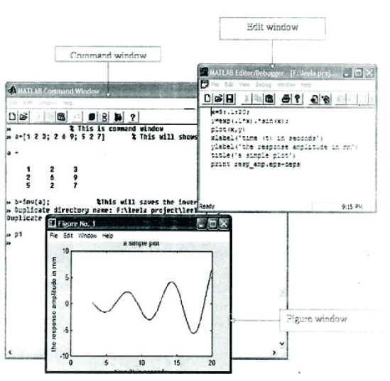
Fig 1.1 The MATLAB Environment Consists of a Command Window, a Figure Window and a Platform-Dependent Edit Window

1. Command Window: This is the main window. It is characterised by the MATLAB command prompt ‘>>’. When we want to develop an application program, MATLAB puts us in this window. All commands, including those for running user-written programs, are typed in this window at the MATLAB prompt.
2. Graphics Window: The output of all graphic commands is typed in the command window or flushed to the graphics or figure window, which is a separate grey window with a (default) white background. The user can create as many figure windows as allowed by the system memory.
3. Edit Window: This is where the user can write, edit, create and save his/her own programs in files called ‘M-files’.

File Types

MATLAB has the following three types of files for storing information.

1. M-files are standard ASCII text files with .m extension to the file name. These files are of two types: script files and function files. Most of the programs written in MATLAB are saved as M-files. All built-in functions in MATLAB are M-files and reside in the computer in a pre-compiled format. Some built-in functions are provided with a source code in readable M-files, so that they can be copied and modified.
2. MAT-files are binary data files, with .mat extension to the file name. MAT-files are created by MATLAB when one saves data using the save command. The data are written in a special format that only MATLAB can read. MAT-files can be loaded into MATLAB with the load command.
3. MEX-files are MATLAB callable FORTRAN and C programs.

Creating, Saving and Executing a Script File

Knowledge of creating a script file is essential. A sequence of MATLAB commands are written in script file. The file shall be saved as an M-file with .m extension. A script file is executed by typing its name without .m extension at the command prompt (>>). The following steps demonstrate the creation, saving and execution of a script file.

Step 1: Click the MATLAB icon, and the MATLAB command window opens.

Step 2: Select ‘New M-file’ from the File menu.

Step 3: Type the lines given below into the file. Lines starting with a % sign are comment lines, which shall be ignored by MATLAB.

Step 4: Save the file as ‘greet_me’.

Step 5: Now get back to MATLAB and type the following commands in the command window to execute the written script file.

>> greet-me

The above command will execute the file that we see on the screen as a greeting message.

To know about MATLAB functions and its other useful features, the reader is referred to use MATLAB User's Guide.