CHAPTER 9

Transient Stability

9.1 Transient Stability—Equal Area Criterion

Equal area criterion (EAC) is the graphical interpretation of transient stability of the system. This method is only applicable to a single machine connected to an infinite bus system or a two-machine system. The concept of EAC is derived from the fact that the stored kinetic energy in the rotating mass tries to substantiate the imbalance between the machine output and input. A single machine connected to a large system such as an infinite bus is considered to explain the EAC concept.

9.1.1 Mathematical Approach to EAC

Consider a synchronous machine connected to an infinite bus. Neglecting the damping effect, the swing equation is rewritten below.

 

 

where P_a is the accelerating power, which is due to imbalance between mechanical input and electrical power output. From the above equation,

 

 

Multiplying both sides of the above equation by 2. we get

 

 

The above equation can be written in the modified form as:

 

 

or

 

 

Integrating both sides,

 

 

or

 

 

Under stable conditions of the machine, the variations in the rotor speed (or ) must be equal to zero. This is possible only when the right hand side terms of Equation (9.3) is zero.

i.e

 

 

The Swing Curve

It is a graph indicating the variations in δ with time t.

 

 

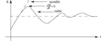
Fig 9.1 Swing Curve for Stable and Unstable Power Systems

 

The swing equation indicates that the rotor shall either accelerate or decelerate when there exists an imbalance between mechanical input and electrical power output. Due to this, the rotor may run above or below the synchronous speed, indicating system instability as shown in Figure 9.1.

Stability/Instability Conditions

 

 

Graphical Interpretation of EAC

Consider the power-angle curve of an alternator as shown in Figure 9.2

Initially the machine is operating at the equilibrium point A, where P_e0 = P_m0 and δ = δ₀ as shown in Figure 9.2. Now, the mechanical input to the machine is suddenly increased from P_m0 to P_m1. As P_m1 > P_c0, the value of accelerating power P_a is positive and hence the rotor starts accelerating. Due to this acceleration of the rotor, δ increases as shown in Fig 9.3.

 

 

Fig 9.2 Power Angle Curve of an Alternator

 

 

Fig 9.3 Rotor Movement from Point A to B

 

With an increase in δ, P_e increases. When δ reaches δ₁ (at point B), the accelerating power P_a becomes zero as P_e = P_m1. At point B, the rotor speed is above synchronous speed and due to inertia it continues to move forward beyond point B. For δ > δ₁, P_e > P_m1, and P_A is negative. Hence the rotor starts decelerating. Beyond point B, the rotor speed is decreases due to deceleration.

The rotor speed reaches N_s at point D. At this point, as P_e > P_m1, the rotor continues to decelerate and δ starts decreasing as shown in Fig 9.4.

 

 

Fig 9.4 Rotor Movement from Point D to B

 

When the rotor reaches point B from D, P_e again equals to P_m1, hence P_a becomes zero. However, due to inertia the rotor continues to move beyond point B towards A and acceleration begins.

The result is that the rotor swings from A to D via B, and from D back to A.

Considering losses (which give damping effect to the rotor), the rotor finally settles down at a new equilibrium point B after performing the swing as explained.

It can be observed that the rotor accelerates when it moves from A to B and decelerates when it is moves from B to D. From the laws of mechanics the machine swings stably when the excess energy stored in the rotating mass while it accelerates is equal to the energy it gives up during deceleration.

Mathematically,

|area A₁| = |area A₂|

 

 

This is known as the equal area criterion.

From EAC, the condition for stability can be stated as follows:

“The accelerating area (positive) under the P − δ curve must be equal to decelerating (negative) area”.

9.1.2 Application of Equal Area Criterion

Now we consider the various types of disturbances on a single machine connected to an infinite bus (SMIB) system and analyse its stability by using the EAC criterion.

Case-1: Mechanical input to the rotor is suddenly increased

Consider the SMIB system shown in Figure 9.5

 

 

Fig 9.5 An SMIB System

 

Electrical power transmitted to the infinite bus is given by

 

 

Initially the system is operating stably, at which

 

 

This initial steady point is marked as point A on the P-δ curve shown in Figure 9.6.

 

 

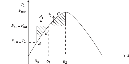
Fig 9.6 Power Angle Curve of an SMIB System for a Sudden Increase in Mechanical Input to the Generator

 

Now, the mechanical input to the generator is suddenly raised to p_m1 from p_m0 by opening the steam valve. Consequent to this change, the following sequence of changes takes place.

Stage-1: At point A

The system is under steady-state with perfect balance between P_m0 and P_e0 and P_a = P_m0 − P_c0 = 0. The speed of the rotor equals to the synchronous speed N_S . Now, the mechanical input to is raised suddenly to P_m1 from P_m0.

Stage-2:Movement from point A to B

Though the mechanical input to the rotor is increased, the generator cannot generate extra electrical power, since δ cannot change instantly due to rotor inertia. Hence, the extra mechanical input P_m1 − P_m0 is stored as kinetic energy within the rotor and therefore the rotor starts accelerating. The speed of the rotor is now above N_S and hence P_e now starts increasing. But the accelerating power begins to reduce as the imbalance between P_m and P_e starts reducing due to an increase in the P_e value.

Stage-3:Reaching point B

On reaching point B, δ value equals to δ₁ and the electrical power output P_e is raised and made equal to P_m1. The rotor now stops accelerating as P_a value is zero. At this point it should be remembered the speed of the rotor is above N_S . Though P_a value is zero, δ continues to increase beyond δ₁ as the forward movement of rotor continues due to inertia of the rotor.

Stage-4:From point B to C

On leaving point B, δ increases beyond δ₁. Due to this, the machine now generates electrical power output more than P_e1. The P_a value is now negative as P_e > P_m1. Due to this the rotor now starts decelerating. It should be noted that though the rotor is decelerating, it still moves in the forward direction (δ increasing) as the speed is more than N_S .

Stage-5:Reaching Point C

On reaching point C, δ value reaches δ₂. Now the speed of the rotor is equal to N_S.

As δ₂ > δ₁, the electrical power output is more than the mechanical input and hence the P_a value is negative. The rotor now decelerates in the reverse direction (δ decreasing) and the negative value of P_a begins to reduce.

Stage-6:From point C to B

On leaving point C, P_e value begins to reduce as δ value is decreasing. This is because the rotor is moving in the backward direction. The decelerating power P_a begins to reduce. However the rotor speed is now lesser than N_S, as the rotor is moving in backward direction.

Stage-7:Reaching point B

On reaching point B, the P_e value becomes equal to P_m1 and hence P_a value is zero. The rotor speed is still less than N_s and the rotor continues to move in the backward direction (δ decreasing) due to inertia.

Stage-8:From point B to A

On leaving point B, δ value becomes less than δ₁, and consequently, P_e value is less than P_m1. Now the P_a value is positive and the rotor begins to accelerate with the rotor speed again starting to increase.

Stage-9:Reaching point A

When the rotor reaches point A, δ value is equal to δ₀ and the rotor speed rises to N_S. It should be understood that while the rotor is moving from point B to A, though its movement is backward it is actually accelerating. Once it reaches the point A, the movement in the backward direction stops and it begins moving in the forward (δ increasing) direction.

This completes one cycle of operation and Stages 1 to 9 are repeated again. If the system damping is considered, these oscillations gradually die out and the machine will settle to the new equilibrium point B

where P_m1 = P_e = P_max sin δ₁

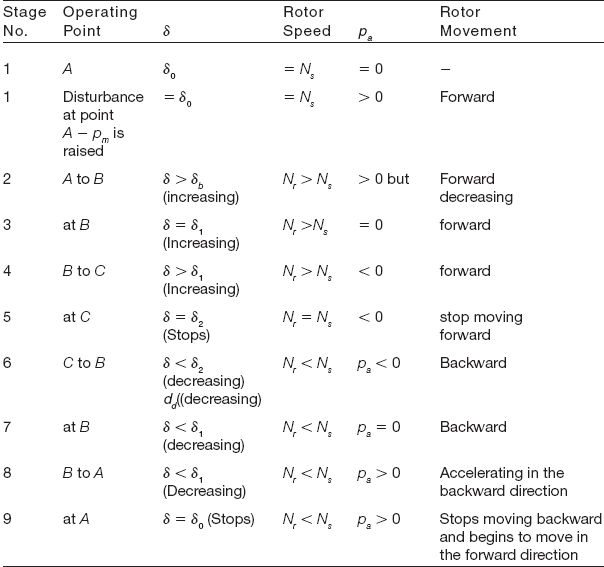
The steps related to the swinging of the rotor are depicted in Table 9.1.

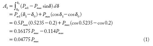
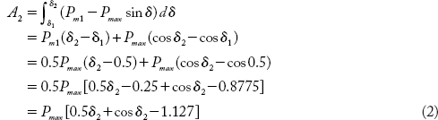
The areas A₁ and A₂ are given by

 

 

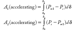
For the system to be stable A₁ = A₂

 

Table 9.1 Steps related to the swinging of the rotor

 

Condition of maximum swing

From the steady-state stability point of view, the system reaches the critical stable point when δ = 90°. However, the system can maintain transient stability beyond δ = 90°, as long as the condition of EAC is satisfied. Figure 9.7 illustrates this.

Limitation to increase in P_m value

Consider the swing curve shown in Figure 9.7.

For the given value of δ₀, an increased value of P_m is such that, if δ goes beyond δ_m the system loses transient stability. At point B, P_e1 = P_m1 = P_max sin δ₁. At point C, P_c1 = P_m1 = P_max sin δ_max. It can be easily verified that the above equations are valid only when δ_max = π − δ₁. Considering the P − δ curve shown in Figure 9.7, if P_m value is increased beyond P_m1 as shown, then the rotor swings beyond δ_m. However, if δ becomes greater than δ_max, then the power transfer will be lesser than P_m and the rotor will experience further acceleration. This will further increase δ and the generator will be out of synchronism (See Figure 9.8).

 

 

Fig 9.7 The System has Transient Stability when the Rotor Swings beyond δ = 90°

 

Fig 9.8 Limiting Case for Increase in P_m

 

Therefore, the limiting value of P_m1 for a given P_m0 can be computed by the condition.

 

 

where

 

 

Case-1: Mathematical Equations for EAC

 

 

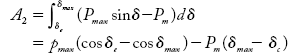
Accelerating area

 

 

Decelerating area

 

 

The system is stable when A₁ = A₂ i.e., p_max(cos δ₀ - cos δ₂) = p_m1(δ₂ - δ₀). Substituting p_m1 = p_e1 = p_maxsin δ₁ in the above equation,

 

 

For the limiting case,

 

 

Therefore,

 

 

For the given value of δ₀, the value of δ₁ cannot be found directly. Equation (9.13) can only solved by the iteration process.

Case-2: Three-Phase Fault on Feeder

Consider Figure 9.9(a) where a generator is connected to an infinite bus bar through a radial feeder.

The p-δ curve is shown in Figure 9.9(b).

Let the system shown in Figure 9.9(a) be operating at point A, where the rotor speed is equal to N_S and δ = δ₀.

Now, a 3-phase fault occurs at point F on one of the outgoing feeders. Since the fault is closer to the generator and as resistance is being neglected, P_e instantly becomes zero. In other words, no electrical power is transferred to the infinite bus.

 

 

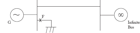
Fig 9.9(a) A Three-Phase Fault at Point F on an SMIB System

 

Fig 9.9(b) p-δ Curve

 

Now, the entire P_m becomes equal to P_a, and the rotor starts accelerating. Since P_e = 0, the operating point shifts immediately to point B and due to rotor acceleration, δ starts increasing. In time t_cr (critical clearing time) when the rotor angle reaches to δ_cr (critical clearing angle), the circuit-breaker installed at point F clears the fault by isolating the faulted line. Upon removal of faulted line, the generator once again starts transmitting power to the infinite bus. Therefore, the operating point shifts from C to D instantly. At point D, since P_e > P_m, the rotor now begins to decelerate and the decelerating area A₂ begins as the operating point moves along D−E.

System is stable as long as A₁ ≤ A₂

9.1.3 Determination of Critical Clearing Angle

For a given initial load there is a maximum value of clearing angle, known as critical clearing angle (δ_cr) for stability to be maintained. If the actual clearing angle δ₁ is smaller than δ_cr, the system is stable. If δ₁ > δ_cr the system is unstable. It should be noted that when δ₁ = δ_cr, the rotor swings up to δ_max, a permitted threshold value. Beyond δ_max, the stability of the system is lost. The circuit-breaker fault clearing time corresponding to δ_cr is known as the critical clearing time (t_cr). If the actual fault clearing time is less than t_cr, the system is stable, otherwise it is unstable.

The formulas for δ_cr and t_cr can be easily derived only for the case when P_e = 0. For other cases it is hard to establish the formulas.

 

 

Fig 9.10 A Simple Case to Determine Critical Clearing Angle δ_cr

 

The following equation can be easily verified in the p-δ curve shown in Figure 9.10

 

 

From the above,

 

 

Now, accelerating area

Since P_e is zero,

 

 

Decelerating area

 

 

For the system to be stable, A₂ = A₁, which yields the following relation

 

 

where δ_cr = critical clearing angle.

By substituting δ_max = π − δ₀ and P_e = P_m = P_maxsin δ₀ in Equation (9.16),

We get,

 

 

Note: The value of δ_cr depend upon initial loading condition of machine. In other words depends on the initial value of δ₀.

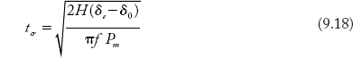
9.1.4 Determination of Critical Clearing Time [t_cr]

During the fault on the system,

 

 

Therefore,

 

 

Substituting

 

 

Integrating the above equation twice,

 

 

From the above,

 

 

Case-3: Loss of Faulted Parallel Line

Consider the power system shown in Figure 9.11. The generator is connected to the infinite bus system through two parallel lines.

 

 

Fig 9.11 Three-Phase Fault occurs at some Point on One Parallel Line of the SMIB System

 

Now, consider a fault at point F some distance away from both ends on one parallel line as shown in Figure 9.11.

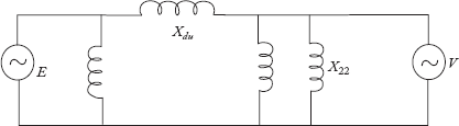
9.1.5 Determination of Transfer Reactance Before, During and After Fault Conditions

 

 

Before fault

 

 

During fault

 

 

Let the transfer reactance during fault be X_du. Its value can be obtained by converting star reactances X^'_d, X₁ and X₂₁ into delta. This is explained in the following figure.

 

 

Post fault:

After some duration, the faulty parallel line is removed by circuit-breakers connected at both ends. The transfer reactance for this condition X_po is:

 

 

The steady-state power limits for these conditions are given below.

1. Before fault
2. During fault
3. Post fault

 

 

Fig 9.12 p–δ Curve for Case-3 Study of EAC

 

Now consider the p-δ curve shown in Figure 9.12.

Assume that the input power P_m is constant and that the machine is operating steadily, delivering power to the infinite bus at δ = δ₀. The p-δ curve for the pre-fault condition is marked as a in the figure. During fault condition, equivalent transfer reactance between bus bars is increased, lowering the steady-state power limit. For this condition the p-δ curve is represented by the curve B. Finally curve C represents the post-fault p-δ curve.

The following sequence of operations takes place.

1. The system is steadily operating at point a

    

   

    

2. Now a fault occurs at point F on one of the parallel line as shown in Figure 9.11. The operating point shifts down to point b on curve B. Due to excess mechanical input, the rotor starts accelerating towards point C.
3. By the time when δ reaches δ_cr, the faulted line is removed from both ends.
4. Now the operating point shifts up from c to e on curve C. Now the rotor begins to decelerate.

System is stable when A₁ (accelerating)

                             = A₂ (decelerating)

i.e., Area a b c d = Area d e f

Applying EAC, for this case δ_e can be obtained as follows,

 

 

where

 

 

Integrating Equation 9.19,

 

 

or

 

 

Case-4: Re-Closure Operation of Circuit Breaker

Considering the fault as temporary, circuit breakers in the faulted line are re-closed after some time. As the fault is cleared, the line is restored into service again.

For this case, p-δ curves for before the fault and after re-closure are the same.

i.e.,

 

 

The p-δ curve is drawn for the case in Figure 9.13.

The stability of the system improves, as the re-closure unit of the circuit breaker restores the second line back into service for transfer of electrical power.

 

 

Fig 9.13 Case-4 of EAC: Application of the Re-Closure Unit

 

The following is the sequence of operations for this case study:

1. Initially the system is operating stably at Point a.

    

   

    

2. A fault occurs at Point F on the radial feeder and the operating point shifts down to Point b. Due to higher value of P_m, the rotor begins to accelerate and δ increases.
3. After some time, the circuit breaker isolates the faulted line. The rotor angle reaches to δ_c. The operating point shifts from c to e, on the post-fault curve C. Since P_e > P_m, the rotor now begins to decelerate.
4. On reaching Point f, when δ = δ_r, the re-closure unit restores the second line back to service. Due to this the operating point shifts from f to g on the pre-fault p-δ curve.
   The accelerating area (A₁) and the decelerating area are (A₂) are marked on the p-δ curve. The maximum angle to which the rotor swings is δ₂ and is less than δ_m (maximum permissible rotor angle). Hence, the system is stable for the condition shown on the p-δ curve.

Example 9.1

A generator is generating 20% of the maximum power it is capable of generating. If the mechanical input to the generator is increased by 250% of the previous value, calculate the maximum value of δ during the swing of rotor around the new equilibrium point.

Solution:

The p-δ curve is shown in Figure 9.14

 

 

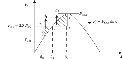
Fig 9.14 P-δ Curve

 

At Point a,

 

 

At Point b,

 

 

Now, we are required to find δ₂.

For the system to be stable,

Accelerating area A₁ = Decelerating area A₂

 

 

Equating (1) and (2),

 

 

The value of δ₂ may be found using the numerical method or the trial and error process. Here δ₂ determined by the trial and error process.

From the condition δ₂ > 0.5235, the starting value of δ₂ is guessed as 0.55

δ2	X = 0.5 δ2 + cos δ2	X - 1.08 = error
0.55	1.1275	0.04752
0.57	1.1269	0.0469
0.6	1.12533	0.04533
0.7	1.1484	0.0348
0.75	1.10668	0.02668
0.77	1.1029	0.0229
0.78	1.10483	0.0248
0.79	1.10091	0.0209
0.8	1.0967	0.016
0.85	1.0849	0.0049
0.86	1.08243	0.00243
0.87	1.0789	0.0001734

From the tabulated results the approximate value of

 

 

Example 9.2

Consider the power system shown in Figure 9.15

 

 

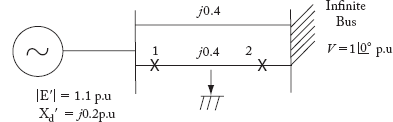
Fig 9.15 An SMIB Power System

 

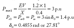
The p.u reactances are marked in the figure. A balanced three-phase fault occurs at the middle point of Line-2. The generator is delivering 1.0 p. u. power at the instant preceding to fault. By the use of equal area criterion, determine the critical clearing angle.

Solution:

Before fault condition:

 

 

During fault condition:

For a fault at the middle of Line-2 the equivalent circuit is as shown in Figure 9.16 below.

Converting star reactances of 0.2, 0.4 and 0.2 p.u into delta, the transfer reactance can be obtained from this equivalent circuit.

 

 

Fig 9.16 Determination of Transfer Reactance

 

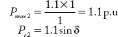
Steady-state power limit for the condition is:

 

 

Post-fault condition:

The fault in Line-2 is removed by opening the circuit breakers at both ends. The transfer reactance for this case is:

 

 

The three power angle curves are shown in Figure 9.17(a).

 

 

Fig 9.17(a) Power Angle Curves for a Fault at the Middle of Line-2

 

Under steady-state conditions prior to fault,

 

 

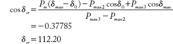
Now, we are required to find δ_cr with 5 reference to Fig 9.17(b)

 

 

Fig 9.17(b) Determination SCR

 

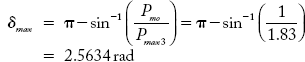
The maximum angle up to which the rotor can swing for a given value of δ₀ is:

 

 

Accelerating area

Decelerating area

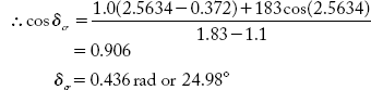
For the system to be stable,

 

 

By integration,

 

 

Solving the above equation,

 

Example 9.3

In the above example, find the critical clearing angle if a three-phase fault occurs on Line-2, close to the generator.

Solution:

In this

 

Example 9.4

Consider the system shown in Figure 9.18.

 

 

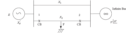
Fig 9.18 An SMIB System

 

The per unit values of different quantities are:

 

 

The system is operating stably with a mechanical input of P_m = 1.4 p.u. Now, one of the lines is suddenly switched off.

1. Comment on the stability of the system
2. If the system is stable, find the maximum value of δ during the swinging of the rotor.

Solution:

1. The p − δ curve for this case is as shown in Figure 9.19.

    

   

    

   Fig 9.19 P—δ Curve

    

   Before Line-2 is switched off:

   Transfer reactance = 0.1 + (0.6||0.6) = 0.4 p.u

    

   

    

   After Line-2 is switched off:

   Transfer reactance = 0.1 + 0.6 = 0.7 p.u.

    

   

    

   As the mechanical input is constant before and after Line-2 is switched off, the generator generates the same amount of electrical power output. The initial equilibrium point is a and the final equilibrium point is c as shown in the figure.

   i.e.,

    

   

    

   From the above, δ₁ can be determined

    

   

    

   Or, δ₁ = 54.77°

   If stability is of interest, the rotor can swing to a maximum of δ_max (up to point f).

   At point c and f, the P_e generated is same.

    

   

    

   Solving, δ_max = π − δ₁ = 2.186 rad or 125.3°

   The accelerating area A₁ is:

    

   

    

   System stability depends on whether or not there is sufficient decelerating area A₂ available. In other words, for the system to stable the condition is A₁ ≤ A₂

   Maximum decelerating area available, A_2,max, can be found as:

    

   

    

   Since A_2max > A₁ the system is stable.

2. The actual value of rotor swing i.e., δ₂ can be found by the condition

    

   

    

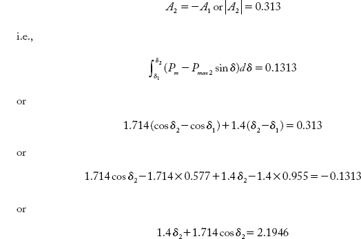
   The above equation cannot be solved directly. Iterative methods are required to obtain δ₂. An approximate value δ₂ is obtained by the trial and error process. The value of δ₂ is such that δ₁ < δ₂ < δ_max.

   i.e.,

    

   

    

   Let us begin with δ₂ = 1.57 rad (approximately the middle point)

    

   

    

   The approximate value of δ₂ = 1.585 rad = 90.82°

9.2 II Solution of the Swing Equation: Point-By-Point Method

There is a need to solve the swing equation for δ as a function of time in order to know the critical clearing time by the numerical technique. The equal-area approach enables us to calculate the critical clearing angle alone.

The evaluation of power system stability can be made effective by solving the swing equation for critical clearing time. This data is used in the design and selection of circuit breakers.

There are various methods available for solving swing equation, including the powerful Range-Kutta method. However, we shall illustrate the conventional and approximate method known as the point-by-point method, which is well-tried and prevalent.

We shall discuss the point-by-point method for one machine connected to the infinite bus bar. The procedure is however general, and can be applied to every machine in a multi-machine system.

Consider the swing equation

 

 

where,

The solution of δ(t) is obtained at discrete intervals of time with the interval spread of Δt remaining uniform throughout. The change in accelerating power which is a continuous function of time is described as follows:

1. The accelerating power P_a calculated at the beginning is assumed to remain constant from the middle of the preceding interval to the middle of the interval under study (see Figure 9.20(a))
2. The angular rotor velocity ( over and above the synchronous velocity ωs, is calculated at the middle of the interval under study, (see Figure 9.20(b)).

      In Figure 9.20(b), the numbering on axis refers to the end of intervals. At the end of the (n − 1)^th interval, the acceleration power is

 

 

Fig 9.20(a-c) Plot of Acceleration, Speed and Rotor Angle: Point-by-Point Method

 

where δ_n−1 has been previously calculated.

The change in velocity ( caused by P_a(n−1), assumed to be constant over Δt from is given as

 

 

The change in δ during the (n − 1)^th interval is

 

 

and during the n^th interval

 

 

Subtracting Equation (9.26) from Equation (9.27) and using Equation (9.25), we get

 

 

Using this, we can write

 

 

The process of computation is now repeated for P_a(n), Δδ_n+1 and δ_n+1.

The time solution in discrete form is worked out for the required length of time, which is normally 0.5 seconds. The solution for the continuous form is obtained by drawing a smooth curve through discrete values as shown in Figure 9.20(c). The solution can be obtained with greater accuracy by reducing the time duration of intervals.

The occurrence or removal of a fault or the initiation of any switching event causes a discontinuity in the accelerating power P_a. If such a discontinuity occurs at the beginning of an interval, then the average of the values of P_a before and after the discontinuity must be used. Thus, for calculating the increment angle occurring during the first interval after a fault is applied, at t = 0 Equation (9.26) becomes,

 

 

where P_ao⁺ is the accelerating power immediately after occurrence of the fault. The system is in steady state just before the occurrence of the fault so that P_ao⁻ = 0 and δ₀ is a known value. If the fault is cleared at the beginning of the n^th interval, for calculating this interval, one has to use for P_a(_n−1) the value is the accelerating power immediately after clearing the fault. If the discontinuity occurs at the middle of the interval, a special procedure is required.

The increment of angle during such an interval is calculated, as usual, from the value of P_a at the beginning of the interval.

The procedure of calculating the solution of a swing equation is illustrated in following example.

Example 9.5

A power system is shown in Figure 9.21

 

 

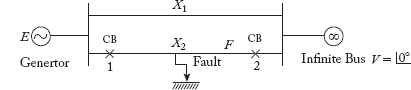
Fig 9.21 Power System for Example 9.5

 

Consider the following data

 

 

The generator is operating stably and supplying 50 MW power to an infinite bus via two transmission lines. Now, a three-phase symmetrical fault occurs at the middle of Line-2.

1. Plot the swing curve if the fault is sustained for 0.5 second.
2. Plot the swing curve if the fault is cleared in 0.1 second by both end circuit breakers.
3. Find the critical clearing angle and the critical clearing time.

Solution:

Taking the rating of the equipment as base, for base MVA = 50, G = 1.0 p.u

 

 

Before fault:

Transfer reactance X = 0.4 p.u

 

 

Under steady-state:

 

 

During fault:

Transfer reactance X = 1.0 p.u

 

 

Post-fault:

Transfer reactance X = 0.6 p.u

 

 

Taking Δt = 0.05 seconds,

 

 

(a) Sustained fault:

A discontinuity exists at t = 0. Therefore, the average value of P_a used at

 

 

All the calculated values are tabulated in Table 9.2.

 

Table 9.2 Calculated δ values for sustained fault

 

A sample calculation at t = 0.1 second is given below.

Sample calculation:

The swing curve is plotted as in Figure 9.22.

 

 

 

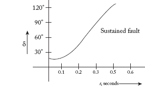
Fig 9.22 Swing Curve for Sustained Fault

 

Table 9.3 Calculated δ values when the fault is cleared in 0.1 second

 

It is evident that the system is unstable.

(b) Fault cleared in 0.1 second:

The swing curve till 0.05 second is the same as that for a sustained fault. As the fault is cleared, P_m changes from 1.05 p.u at t = 0.10⁻ to 1.75 p.u at t = 0.10₊. Since the discontinuity occurs at the beginning of an interval, it is required to calculate the average value of P_a at t = 0.1 second and use this value in computing Δδ at this time. The procedure for computing the values remains the same as before.

 

 

Fig 9.23 Swing Curve for a Fault Cleared in 0.1 Second

 

Through tabulated results it can be concluded that the system is stable.

(c)

 

 

Using the equation,

 

9.3 Methods to Improve Transient Stability

The following methods can be used to improve transient stability:

1. Increase of system voltage:

   It is important to note that the steady-state stability limit is always higher than the transient stability limit. Systems having higher steady-state stability limits are generally guaranteed for better transient stability. However, though inertia of the machine plays a vital role in transient stability, the converse is not true. By improving steady-state power limit, it can be seen in the p-δ curve that the rotor can swing in such a way that it can attain higher accelerating and decelerating areas. With this, transient stability can be improved. The value of P_max in the p-δ curve is directly proportional to the internal voltage E of the machine. An increase in voltage increases the stability limit.

2. Increase in inertia of the machines:

   A heavy-weight machine has higher inertia and is more stable than a light-weight machine. This can be verified through the swing equation as:

    

   

    

   If the machine has a higher inertia constant M, then during the transient period the rotor cannot swing for higher δ values. Generally a salient pole machine swings for lower load angles and is preferred over cylindrical rotor generators. The present practice of generating higher power with larger number of small machines is not recommended from the stability point of view.

3. Quick-acting governors:

   The instability of a system is mainly due to excess kinetic energy stored in the rotating mass during disturbance. The problem can be avoided if the prime mover (turbine) output is quickly adjusted. This requires quick valve opening and closing action of the speed-governing system. This method is quite difficult to be implemented with conventional mechanical governors since they are too slow to respond on account of their high time constants. Electronically operated governors may be suggested for this purpose.

4. Quick-responding excitation systems:

   Whenever a fault occurs in a system, reactive power demand increases while there is a reduction in active power generation. Reduction in active power is mainly due to a rapid dip in terminal voltage as the generator experiences demagnetization armature reaction. Fast-field excitation systems quickly respond to the situation and improve the electric power output of generator, reducing the acceleration of the rotor during the disturbance period. Thus exciters help to improve the stability of the system.

5. Reduction in transfer reactance:

   As stated earlier, systems having better steady-state stability margins are guaranteed for better transient stability limits. By reducing transfer reactance, steady-state power limit can be improved. Reduction in transfer reactance can be achieved by:

   1. using bundled conductors
   2. using conductors with larger diameter
   3. using series capacitors.
6. Use of high-speed circuit breakers:

   As seen in Section 9.1, if the circuit breaker clears the fault before the critical clearing time, the system can maintain transient stability.

7. Use of auto re-closing circuit breakers:

   Most of the faults that occur in a system are temporary in nature. Auto re-closing circuit breakers connect the faulted lines back into service after the fault has disappeared in the system. This improves the power transfer capability, and thereby the stability of the system.

8. Single-pole switching circuit breakers:

   A majority of faults occurring in a system are of the single-line to ground type. If the circuit breaker is equipped with single-pole switching facility, the faulted single phase can be isolated and switched off. Power generation cannot be zero in this case and hence the stability improves. However, prolonged operation of generator with less number of phases is not advisable. Necessary precautions should be taken to counter this problem.

9. Use of breaking resistors:

   When a fault occurs in a generator, breaking resistors are automatically inserted across the generator terminals. The generator continues to generate power treating these resistors as load. The imbalance between mechanical input and power output is reduced, and hence the system shall be able to maintain stability.

Questions from Previous Question Papers

1. List the assumptions made in the transient stability solution techniques.
2. What is the swing equation? Derive the expression for swing equation?
3. Device and explain the concept of equal area criterion for stability analysis of a power system.
4. What are the factors that affect transient stability?
5. What is equal area criterion? Explain how it can be used to study stability?
6. Draw a diagram to illustrate the application of equal area criterion to study transient stability when there is a sudden increase in the input of generator.
7. Discuss the limitations of equal area criterion of method of stability study.
8. Draw the diagrams to illustrate the application of equal area criterion to study transient stability for the following cases:
   1. A switching operation causing the switching out of one of the circuits of a double circuit line feeding an infinite bus.
   2. A fault on one of the parallel circuits of a two-circuit line feeding an infinite bus. The fault is very close to the sending end bus and is subsequently cleared by the opening of the faulted line.
9. What are the methods used to improve the transient stability limit?
10. Discuss the methods to improve steady state and transient state stability margins.
11. Discuss why?

    the use of automatic enclosing circuit breakers improve system stability.

12. A generator is delivering 1 p.u. power to infinite bus system through a purely reactive network. A fault occurs on the system and reduces the output is zero. The maximum power that could be delivered is 2.5 p.u. When the fault is cleared, the original network conditions exist again. Compute the critical clearing angle.
13. (a) A generator operating at 50Hz delivers 1 p.u. power to an infinite bus through a transmission circuit in which resistance is ignored. A fault takes place reducing the maximum power transferable to 0.5 p.u. whereas before the fault this power was 2.0 p.u., and after the clearance of the fault it is 1.5 p.u. By the use of equal area criterion determine the critical clearing angle.

    (b) Derive the formula used in the above problem.

14. Discuss how equal area criterion can be employed for determining the critical clearing angle.
15. A generator operating at 50Hz delivers 1 p.u. power to an infinite bus through a transmission circuit in which resistance is neglected. A fault takes place reducing the maximum power transferable to 0.3 p.u., whereas before the fault this power was 2.0. p.u. and after the clearance of the fault it is 1.5. p.u. By the use of equal area criterion determine the critical clearing angle.
16. Exaplain the point-by-point method for solving the swing equation.

Competitive Examination Questions

1. A generator is supplying 1 per unit power to an infinite bus through the system shown in figure. Following a fault at F, circuit breakers B₃ and B₄ open simultaneously. The P − δ relationships in per unit are given by

   Pre-fault condition: p = 2 sin δ

   During fault condition: When B₃, B₄ remain closed: p = 0.2 sin δ After B₃, B₄ open: p = 1.5 sin δ

   Calculate the critical angle δ before which breakers B₃ and B₄ must open so that synchronism is not lost. Also show this on a P − δ diagram.

    

   [GATE 1991 Q.No. 8]

    

   

    

2. The transient stability of the power system can be effectively improved by
   1. excitation control
   2. phase shifting transformer
   3. single pole switching of circuit breakers
   4. increasing the turbine valve opening

    

   [GATE 1993 Q.No. 3]

3. During a disturbance on a synchronous machine, the rotor swings from A to B before finally settling down to a steady state at point C on the power angle curve. The speed of the machine during oscillation is synchronous at point(s)
   1. A and B
   2. A and C
   3. B and C
   4. only at C

    

   [GATE 1995 Q.No. 1]

4. A generator is delivering rated power of 1.0 per unit to an infinite bus through a lossless network. A three-phase fault under this condition reduces P_max to 0 per unit. The value of P_max before fault is 2.0 per unit and 1.5 per unit after fault clearing. If the fault is cleared in 0.05 seconds, calculate rotor angles at intervals of 0.05 seconds from t = 0 seconds to 0.1 seconds. Assume H = 7.5 HJ/MVA and frequency to be Hz.

    

   [GATE 1996 Q.No. 13]

5. A 100 MVA,11 kV, 3-phase, 50 Hz, 8-pole synchronous generator has an inertia constant H equal to 4 seconds. The stored energy in the rotor of the generator at synchronous speed will be H = E/G.
   1. 100 MJ
   2. 400 MJ
   3. 800 MJ
   4. 12.5 MJ

    

   [GATE 1997 Q.No. 4]

6. The use of high-speed circuit-breakers
   1. Reduce the short circuit current
   2. Improve system stability
   3. Decrease system stability
   4. Increase the short circuit current

    

   [GATE 1997 Q.No. 5]

7. A power station consists of two synchronous generators A and B of ratings 250 MVA and 500 MVA with inertia 1.6 p.u. and 1 p.u., respectively on their own base MVA ratings. The equivalent p.u. inertia constant for the system on 100 MVA common base is:
   1. 2.6
   2. 0.615
   3. 1.625
   4. 9.0

    

   [GATE 1998 Q.No. 7]

8. An alternator is connected to an infinite bus as shown in figure. It delivers 1.0 p.u. current at 0.8 pf lagging at V = 1.0 p.u. The reactance X_d of the alternator is 1.2 p.u. Determine the active power output and the steady state power limit. Keeping the active power fixed, if the excitation is reduced, find the critical excitation corresponding to operation at stability limit.

    

   [GATE 1998 Q.No. 12]

    

   

    

9. A synchronous generator, having a reactance of 0.15 p.u., is connected to an infinite bus through two identical parallel transmission lines having reactance of 0.3 p.u. each. In steady state, the generator is delivering 1 p.u. power to the infinite bus. For a three-phase fault at the receiving end of one line, calculate the rotor angle at the end of first time step of 0.05 seconds. Assume the voltage behind transient reactance for the generator as 1.1 p.u. and infinite bus voltage as 1.0 p.u. Also indicate how the accelerating powers will be evaluated for the next time step if the breaker clears the fault
   1. at the end of an interval
   2. at the middle of an interval

    

   [GATE 2000 Q.No. 14]

10. A synchronous generator is connected to an infinite bus through a lossless double circuit transmission line. The generator is delivering 1.0 per unit power at a load angle of 30° when a sudden fault reduces the peak power that can be transmitted to 0.5 per unit. After clearance of fault, the peak power that can be transmitted becomes 1.5 per unit. Find the critical clearing angle.

     

    [GATE 2001 Q.No. 13]

11. A synchronous generator is to be connected to an infinite bus through a transmission line of reactance X=0.2 pu, as shown in figure. The generator data is as follows:

    x^′ = 0.1p.u, E^′ = 1.0p.u, H = 5MJ/MVA, mechanical power Pm = 0.0p.u, ω_B = 2π × 50 rad/sec. All quantities are expressed on a common base.

     

    [GATE 2002 Q.No. 10]

    The generator is initially running on open circuit with the frequency of the open circuit voltage slightly higher than that of the infinite bus. If at the instant of switch closure δ = 0 and ω = dδ/dt = ω_init, compute the maximum value of ω_init so that the generator pulls into synchronism.

    Hint: Use the equation

     

    

     

12. A generator delivers power of 1.0 p.u. to an infinite bus through a purely reactive network. The maximum power that could be delivered by the generator is 2.0 p.u. A three-phase fault occurs at the terminals of the generator which reduces the generator output to zero. The fault is cleared after t_c second. The original network is then restored. The maximum swing of the rotor angle is found to be δ_max = 110 electrical degree. Then the rotor angle in electrical degrees at t = t_c is
    1. 55
    2. 70
    3. 69.14
    4. 72.4

     

    [GATE 2003 Q.No. 15]

13. A 50 Hz, 4-pole, 500 MVA, 22 kV turbo-generator is delivering rated megavolt amperes at 0.8 power factor. Suddenly a fault occurs reducing is electric power output by 40%. Neglect losses and assume constant power input to the shaft. The accelerating torque in the generator in MNm at the time of the fault will be
    1. 1.528
    2. 1.018
    3. 0.848
    4. 0.509

     

    [GATE 2004 Q.No. 14]

14. A generator feeds power to an infinite bus through a double circuit transmission line. A 3-phase fault occurs at the middle point of one of the lines. The infinite bus voltage is 1 pu, the transient internal voltage of the generator is 1.1 pu and the equivalent transfer admittance during fault is 0.8 pu. The 100 MVA generator has an inertia constant of 5 MJ/MVA and it was delivering 1.0 pu power prior to the fault with rotor power angle of 30°. The system frequency is 50 Hz.

    (A) The initial accelerating power (in p.u) will be

    1. 1.0
    2. 0.6
    3. 0.56
    4. 0.4

     

    [GATE 2006 Q.No. 13]

15. If the initial accelerating power is X p.u, the initial acceleration in elect deg/sec², and the inertia constant in MJ-sec/elect deg respectively will be
    1. 31.4X, 18
    2. 1800X, 0.056
    3. X/1800, 0.056
    4. X/31.4, 18

     

    [GATE 2006 Q.No. 14]

16. A lossless single machine infinite bus power system is shown below

     

    

     

    The synchronous generator transfers 1.0 per unit of power to the infinite bus. Critical clearing time of circuit breaker is 0.28 s. If another identical synchronous generator is connected in parallel to the existing generator and each generator is scheduled to supply 0.5 per unit of power. Then the critical clearing time of the circuit breaker will

    1. reduce to 0.14 s
    2. reduce but will be more than 0.14 s
    3. remain constant at 0.28 s
    4. increase beyond 0.28 s

     

    [GATE 2008 Q.No. 53]