
4
Dimensional Analysis
4.1. Introduction
Various physical phenomena of interest to engineering are described by a number of magnitudes, laws and equations that sometimes involve several parameters. The values of these parameters define the state of the system (Langhaar, 1951).
For example, we saw in Chapter 2 that the magnitude “heat flux transmitted by conduction” depends on a closely-defined set of parameters: the heat conductivity of the material considered, the transfer area and the temperature gradient.
Yet, generally speaking, when we come to study a phenomenon for the first time, in principle we do not tend to know the set of parameters concerned. We therefore apply common sense and physical analysis of the transformations underway, in order to deduce the parameters that could potentially influence the phenomenon being studied.
Nevertheless, this physical analysis is often not enough to be able to determine all of the parameters that can be involved, all the more so when defining the relation that has to exist between these parameters and the magnitude studied.
Put simply, dimensional analysis is, firstly, a technique for defining the dimensions (temperature, length, mass, time, etc.) occurring in a given magnitude. Velocity, for example, involves the dimensions “length” and “time”. Secondly, this technique can be be used to reveal the relations that describe a given physical phenomenon.
Dimensional analysis is thus used as a mathematical technique to methodically explore the parameters that might condition a physical operation. The aim is to uncover the complete set of parameters involved in the quantitative description of this phenomenon, along with the way in which these parameters combine in a magnitude, thus giving the equation that quantitatively represents the physical transformation being studied.
This method of analysis is based on a simple concept: every magnitude and every parameter has a certain number of base dimensions (Porter, 1933).
4.2. Basic dimensions
We already know that all magnitudes and physical parameters admit units and dimensions. We also know that the units of a magnitude are expressed differently according to the system of measurement used (IS, Anglo-Saxon, etc.). The dimensions of a magnitude, on the other hand, are universal and depend only on a limited set (Bridgman, 1937), called basic dimensions.
Table 4.1 gives a set of basic dimensions that can be used to represent the magnitudes used in energy and mass transfers.
Table 4.1. Basic dimensions
| Basic dimensions | Symbol |
| Length | [L] |
| Mass | [M] |
| Time | [t] |
| Electric current | [I] |
| Electrical charge | [C] |
| Temperature | [θ] |
| Light intensity | [φ] |
| Matter amount | [mol] |
4.3. Dimensions of derived magnitudes
Each of the magnitudes that we use (also called derived magnitudes) has an expression (formula), which links it to the parameters conditioning it. Likewise, each parameter, for example, the temperature or transfer area, admits basic dimensions.
The dimensions of the derived magnitudes are determined from the base dimensions of the parameters involved in the definition of these magnitudes; for example:
- – A velocity is a derived magnitude with the dimension of a length per unit time; this is expressed as follows: [v] = [L] [t]-1.
- – An acceleration is a derived magnitude with the dimension of a length by the square of time: [γ] = [L][t]-2.
- – A force can be expressed as a mass multiplied by an acceleration. This enables the dimensions of a force to be determined: [Force] = [M] [L] [t]- 2.
- – An energy can be expressed as the product of a mass by the square of a velocity; hence its dimensions: [Energy] = [M] [L]2[t]-2.
Table 4.2 presents the dimensions of several standard derived magnitudes.
Table 4.2. Dimensions of several derived magnitudes
| Magnitude | Symbol | Dimensions |
| Angular acceleration | θ | [t]-2 |
| Acceleration of gravity | G | [L] [t]-2 |
| Sensible heat | Cp | [L]2 [t]-2 [θ]-1 |
| Volumetric expansion coefficient | β | [θ]-1 |
| Global exchange coefficient | U | [M] [t]-3 [θ]-1 |
| Local exchange coefficient | h | [M] [t]-3 [θ]-1 |
| Mass concentration | c | [M] [L]3 |
| Molar concentration | c | [mol] [L]3 |
| Heat conductivity | λ | [M] [L] [t]-3 [θ]-1 |
| Mass flow rate | W, Γ | [M] [t]-1 |
| Molar flow rate | [mol] [t]-1 | |
| Temperature difference | ∆θ or ∆T | [θ] |
| Thermal diffusivity | α | [L]2 [t]-1 |
| Energy | E, Q | [M] [L]2 [t]-2 |
| Energy flux | φ | [M] [L]2 [t]-3 |
| Force or weight | F or P | [M] [L] [t]-2 |
| Electric current intensity | I | [I] |
| Molar mass | M | [M] [mol] -1 |
| Density | Ρ | [M][L]-3 |
| Modulus of elasticity | E | [M] [L] -1 [t]-2 |
| Modulus of inertia | Z, W or I/ν | [L]3 |
| Moment of inertia | J or I | [M] [L]2 |
| Moment of a force or torque | M or T | [M] [L] 2 [t]-2 |
| Pressure, normal or tangential stress | P, σor τ | [M] [L] -1 [t]-2 |
| Power | P | [M] [L]2 [t]-3 |
| Electrical resistance or impedance | R | [M] [L]2 [t]-3 [I]-2 |
| Electromotive voltage or force | U or E | [M] [L]2 [t]-3 [I]-1 |
| Work or energy | W or E | [M] [L]2 [t]-2 |
| Kinematic viscosity | ν | [L] 2 [t] |
| Dynamic viscosity | µ | [M] [L] -1 [t]-1 |
| Angular velocity | ω | [t]-1 |
4.4. Dimensional analysis of an expression
One of the direct applications of dimensional analysis is the verification of the validity of a given equation, linking a given magnitude to the parameters that condition it. Indeed, it can be extremely useful to analyze the dimensional structure of an equation: as well as serving to verify the validity of the expression given by an equation, it can also be used to determine the dimensions or units of the parameters involved. The following examples illustrate this type of use.
4.4.1. Illustration: determining the dimensions of λ
Question
From the expression of Fourier’s law, determine the dimensions of heat conductivity.
Solution
Let us recall Fourier’s law: 
We know that:
hence the dimensional equation: ![]()
Therefore: ![]()
4.4.2. Illustration: determining the dimensions of h
Question
From the convection equation, determine the dimensions of the convection heat transfer coefficient.
Solution
Let us recall the convection equation:

Hence the dimensional equation: ![]()
Therefore: ![]()
4.5. Unit systems and conversions
It is very important to differentiate between the dimensions of a magnitude and its units. As we have seen, the dimensions define the structure of this magnitude, with respect to the basic dimensions. The units, for their part, enable the magnitude to be assessed with respect to a given measurement system (e.g. IS).
We also know that several measurement systems exist (IS, English, American, etc.) and that each of these systems observe well-defined standards.
The same magnitude can therefore take different values in different measurement systems, whereas its dimensions have one sole expression.
It is therefore important to differentiate between the dimensions of a given magnitude G on the one hand, and its units on the other hand. Indeed, we will use different notations for the dimensions of a magnitude G and its units:
- – To indicate the dimensions of G, we will write: [G].
- – To indicate the units of G, we will write:
 .
.
Dimensional analysis may be used to to determine or validate the coherent set of units that need to accompany a given magnitude. The following examples help illustrate this usage.
4.5.1. Illustration: dimensions and units of energy
We have seen that energy, as a derived magnitude, admits the dimensional structure given in Table 4.2., which uses the base dimensions, [M], [L] and [t].
Thus, the dimensional equation of energy is written as follows:
Of course, this expression does not depend on the system of units used; it is the same for any system of units, as it is solely linked to the base dimensions and to the structure of the magnitude considered.
We know that energy, on the other hand, may be expressed in joules or in calories, etc.
The following table presents the different energy units which are possible using different standard systems.
4.5.2. Illustration: units of heat conductivity λ
Question
From these heat conductivity dimensions, determine the units of λ in the following systems: IS, industrial and Anglo-Saxon.
Solution
In section 4.4.1 we saw that the dimensional equation of λ is written as follows:
In order to be able to deduce the units of λ in a coherent system of units, the dimensional groups corresponding to known magnitudes (energy, acceleration, area, temperature, etc.) need to be shown in the dimensional expression of λ.
The structure of the term [M] [t]-3 [L], which appears in the dimensions of λ, is similar to that of a power. Indeed:
It is therefore possible to identify a power in the dimensional structure of [λ] as follows:

i.e.: ![]()

The following table gives the units of λ in different systems.
| System of units | |
| IS | W/m °C |
| Industrial | Cal/s m °C or kcal/hr m °C |
| Anglo-Saxon | Btu/hr ft °F |
The unit kcal/h m °C is the most commonly used in industry.
The tables presented at the end of this book (see Appendix) present conversion factors between the most commonly used systems of units, along with the definitions of certain Anglo-Saxon units.
4.5.3. Illustration: units of the convective transfer coefficient h
Question
From the convective transfer coefficient dimensional equation, determine the units of this coefficient in the following systems: IS, industrial and Anglo-Saxon.
Solution
By conducting a dimensional analysis on the law of convection we can show that the dimensional equation of coefficient h is given by:
Yet, [M][t]-3 is a power per unit area.
Hence: 
The following table gives the units of h in different systems.
Table 4.5. Units of the convection heat transfer coefficient, h
| System of units | |
| IS | W/m2 °C |
| Industrial | Cal/s m2 °C or kcal/h m2 °C |
| Anglo-Saxon | Btu/h ft2 °F |
A coherent set of units of h could therefore be J/(s m2 °C) or, alternatively, W/(m2 °C).
The unit kcal/h m °C is the most commonly used in industry.
The tables given at the end of this book (see Appendix) present conversion factors for the coefficient h between different systems of units.
4.6. Dimensionless numbers
The parameters conditioning transfer processes, including the exchange of heat, mass or momentum (fluid mechanics), are often clustered together into dimensionless groups (or non-dimensional numbers). This is done, inter alia, with the aim of reducing the number of variables conditioning a given magnitude to a small set of groups of parameters. This reduction is of major importance when we have to determine by experimentation the expressions linking the magnitudes considered to the parameters conditioning them. Indeed, as we will see in the following sections, this reduces the number of experiments having to be conducted in the laboratory in order to study a given physical phenomenon.
It is obvious that, if the expression defining a magnitude G is to be experimentally determined, as a function of a set of parameters (pi 1 ≤ i ≤ n), then the larger the number of parameters involved, the more experiments need to be conducted. The grouping of some of these parameters into dimensionless groups thus makes it possible to significantly reduce the number of variables that are to be studied.
Moreover, the grouping of dimensional parameters into dimensionless numbers makes it possible not to worry about units in formulas and laws.
The dimensionless numbers usually used to describe transfer phenomena are presented briefly below (Boucher & Alves, 1960).
4.6.1. The Reynolds number
This is defined by: ![]()
where:
- d is the inner diameter of the tube, in which the flow occurs.
- v is the velocity of the liquid flowing in the tube.
- ρ designates the density of the flowing fluid.
- μ is the dynamic viscosity of the fluid.
Using the Reynolds number, we can determine the nature of a fluid flow:
- – The flow is said to be “laminar” when Re ≤ 2,300: the fluid flows in parallel layers.
- – The flow is said to be “turbulent” when Re > 4,000: the fluid flows in an irregular manner, which nevertheless leads to an overall defined displacement of the fluid.
- – When 2,300 < Re ≤ 4,000, the flow is said to be “transitional”.
4.6.2. The Nusselt number
This is defined by: ![]()
where:
- h is the convective heat transfer coefficient.
- d is the inner or outer diameter of the pipe.
- λ designates the heat conductivity of the flowing fluid.
The Nusselt number may be considered as a measurement of the ratio between the heat flux transferred by convection and that transmitted by conduction.
4.6.3. The Prandtl number
This is defined by: ![]()
where:
- Cp is the specific heat of the fluid.
- μ is the viscosity of the fluid.
- λ designates the heat conductivity of the flowing fluid.
We can also write: ![]()
Yet: ![]()
Hence: ![]()
Therefore, the Prandtl number is the ratio of the kinematic viscosity ν (which represents diffusivity for momentum transfer) to thermal diffusivity α.
4.6.4. The Peclet number
This is defined by: ![]()
where:
- d is the inner diameter of the tube in which the flow occurs.
- v is the average velocity of the fluid.
- ρ is the density of the fluid.
- Cp is the specific heat of the fluid.
- λ is the heat conductivity of the flowing fluid.
The Peclet number can then be considered as the ratio of the flux of thermal energy transported by the fluid in motion, to the flux of thermal energy transferred by conduction.
It can be noted that: 
Hence: ![]()
4.6.5. The Grashof number
This is defined by: 
where:
- L is the characteristic dimension of the area considered.
- ρ is the density of the fluid.
- g is the acceleration of gravity.
- β is the volumetric expansion coefficient of the constant-pressure fluid.
- ∆ θ is the difference between the wall temperature and the average fluid temperature.
- μ is the viscosity of the fluid.
The Grashof number characterizes the motion of the fluid caused by temperature variations (natural convection). It is analogous to the Reynolds number for forced flow.
4.6.6. The Rayleigh number
This is defined by: Ra = Gr Pr
i.e.: ![]()
This is defined by: ![]()
where:
- L is the characteristic dimension of the area considered.
- ρ is the density of the fluid.
- g is the acceleration of gravity.
- β is the volumetric expansion coefficient of the constant-pressure fluid.
- ∆ θ is the difference between the wall temperature and the average fluid temperature.
- λ is the heat conductivity of the flowing fluid.
- μ is the viscosity of the fluid.
4.6.7. The Stanton number
where:
- h is the convection heat transfer coefficient.
- Cp is the specific heat of the fluid.
- v is the average velocity of the fluid.
- ρ is the density of the fluid.
It measures the significance of the overall heat flux transferred into the fluid, relative to the heat flux transported by the fluid in motion.
We can easily demonstrate that: ![]()
Indeed: 
4.6.8. The Graetz number
This is defined by:
where:
- W is the fluid mass flow rate.
- Cp is the specific heat of the fluid.
- λ designates the heat conductivity of the flowing fluid.
- L is the characteristic dimension of the area considered.
It measures the ratio between the heat flux transported by the fluid and the heat flux transferred by conduction.
4.6.9. The Biot number
This is defined by:
where:
- h is the convective heat transfer coefficient between the liquid and the solid.
- s is a characteristic dimension of the solid considered.
- λ designates the heat conductivity of the solid considered.
It gives the relative importance of convection with respect to conduction.
4.6.10. The Fourier number
This is defined by:

where:
- α is the thermal diffusivity of the material considered, defined by

- t designates the time.
- s is a characteristic dimension of the solid considered.
It gives an idea of the rapidity of heat transfer in a solid.
4.6.11. The Elenbaas number
This is defined by: ![]()
where:
- L is the length of the base comprising fins.
- z is the distance between two fins.
- ρ is the density of the fluid.
- β is the volumetric expansion coefficient of the constant-pressure fluid.
- g is the acceleration of gravity.
- ∆ θ is the difference between the wall temperature of the fins and the temperature of the fluid at large.
- Cp is the specific heat of the fluid.
- μ is the viscosity of the fluid.
It gives an idea of the importance of natural convection with respect to viscosity forces.
4.6.12. The Froude number
This is defined by:

where:
- v is the average velocity of the fluid.
- g is the acceleration of gravity.
- L is the length of the tube considered.
It gives an idea of the energy transported by a fluid circulating at velocity v, with respect to the friction forces due to gravity over a length L.
4.6.13. The Euler number
This is defined by:

where:
- ΔP is the pressure drop due to the flow of a fluid at velocity v.
- ρ is the density of the fluid.
- v is the average velocity of the fluid.
It gives an idea of the load losses due to flow with respect to the energy transported by a fluid circulating at velocity v.
Table 4.6 presents a summary of dimensionless numbers.
Table 4.6. Dimensionless numbers
| Number type | Expression | Parameter description |
| Reynolds | d: inner diameter of the tube v: velocity of the fluid ρ: density of the fluid μ: viscosity of the fluid |
|
| Nusselt |  | h: convective heat transfer coefficient d: inner or outer diameter of the tube λ: heat conductivity of the fluid |
| Prandtl |  |
Cp: specific heat of the fluid μ: viscosity of the fluid λ: heat conductivity of the fluid ν: kinematic viscosity: ν = μ/ρ α: thermal diffusivity: α = λ/ρCp |
| Peclet |  | d: inner diameter of the tube v: velocity of the fluid ρ: density of the fluid Cp: specific heat of the fluid λ: heat conductivity of the fluid |
| Grashof |  | L: characteristic dimension of the area ρ: density of the fluid g: acceleration of gravity β: volumetric expansion coefficient of the constant-pressure fluid ∆θ: difference between the wall temperature and the average fluid temperature μ: viscosity of the fluid |
| Stanton |  | h: convective heat transfer coefficient ρ: density of the fluid Cp: specific heat of the fluid v: velocity of the fluid ρ: density of the fluid |
| Graetz |  | W: mass flow rate of the fluid Cp: specific heat of the fluid λ: heat conductivity of the fluid L: characteristic dimension of the area |
| Biot |  |
h: convective heat transfer coefficient s: characteristic dimension of the solid considered λ: heat conductivity of the solid considered |
| Fourier |  | α: thermal diffusivity: α = λ/ρCp λ: heat conductivity of the solid considered ρ: density of the solid considered Cp: specific heat of the solid considered t: time s: characteristic dimension of the solid considered |
| Elenbaas |  | L: length of the base comprising fins z: distance between two fins ρ: density of the fluid β: fluid expansion coefficient G: acceleration of gravity ∆θ: Twall - T∞ Cp: specific heat of the fluid μ: viscosity of the fluid. |
| Froude | v: average velocity of the fluid g: acceleration of gravity L: length of the tube considered |
|
| Euler |  |
ΔP: load loss due to the flow of a fluid at velocity v ρ: density of the fluid v: average velocity of the fluid |
4.7. Developing correlations through dimensional analysis
When the equation defining the relation between a magnitude G and its variables vi(1 ≤ i ≤ n) cannot be derived analytically through theoretical developments, we generally resort to establishing correlations based on experimental data. A correlation is an equation defining the magnitude G as a function of the variables of the problem, vi(1 ≤ i ≤ n):
Note that, in the simplest case, where theoretical analysis shows that the magnitude G depends on a single variable v it is possible to determine the correlation between G and v simply by means of one experiment, during which v is made to vary and the resulting values of G are noted (see Figure 4.1).

Figure 4.1. Magnitude depending on a single variable
If, on the other hand, preliminary theoretical analysis shows that the magnitude G depends on two variables, then the problem becomes more complex. Indeed, it will be necessary, in this case, to conduct two series of experiments: one with constant v2 (measuring G for different values of v1) and the other with constant v1 (measuring G for different values of v2) (see Figures 4.2 (a) and (b)).

Figure 4.2(a). Magnitude G depending on two variables, v1 and v2 (v2 constant)

Figure 4.2(b). Magnitude G depending on two variables, v1 and v2 (v1 constant)
We can therefore imagine the number of experiments to be carried out if the magnitude G was correlated by several variables. This is often the case for engineering problems.
Using dimensional analysis makes it possible to reduce the number of variables, and therefore the number of experiments, by using Rayleigh's method and the Buckingham theorem.
4.8. Rayleigh’s method
Consider that a magnitude G may be described by the n variables: v1, v2, …, vn.
In general (Rayleigh, 1915), this dependance can be written as:

where A is a dimensionless constant, but the exponents, αi, must be such that the dimensional homogeneity of the equation defining G is ensured.
Thus, assuming that the magnitude G and the different variables are functions of m basic dimensions, [d1], [d2], …, [dm], and given that A is dimensionless, we have:

and: 
The dimensional homogeneity of equation [4.1] will therefore imply:

Since A is dimensionless, the different multiplications that appear in the second member of this equation can be rearranged into a single product. We will then have:

Since the basic dimensions are independent, this equality can only be satisfied if the exponents relative to each dimension, dk, are equal for the two sides of the equality; that is to say:
Or, more explicitly:

We thus obtain a system of m equations, linking the n unknown αi values.
Thus, if a magnitude G and its n variables are expressed using m basic dimensions, then there are at most m relations that must be satisfied by the Δi exponents of G and the αj exponents of the vj variables.
This property enables the number of unknown parameters (αj for 1 ≤ j ≤ n) to be reduced from n to n-m.
4.8.1. Illustration: applying Rayleigh’s method
In fluid mechanics, it is demonstrated that the pressure drop ΔP due to the flow of a fluid of viscosity μ in a pipe of inner diameter d depends on the following parameters:
- – The flow velocity of the fluid: v.
- – The density of the fluid: ρ.
- – The viscosity of the fluid: μ.
- – The roughness of the inside walls of the pipe: ε.
- – The pipe length: 1.
- – The pipe diameter: d.
- – The acceleration of gravity: g.
Questions
1) Give the basic dimensions of the magnitude ΔP and those of the different variables that condition it.
2) We will write ΔP in the form: ![]() ; what, therefore,
; what, therefore,
is the maximum number of equations to be satisfied by the parameters Δi of G and the exponents αj of variables vj?
3) Write the equation that conveys dimensional homogeneity.
4) Deduce the system of equations that must be satisfied by the exponents αj of variables vj.
Solutions
1) Basic dimensions of ΔP and of the variables conditioning it.
ΔP has the dimensions of a pressure.
Therefore: ![]()
Moreover, the dimensions of the different variables occurring in the definition of ΔP are:

2) Maximum number of equations between parameters
Note that the seven variables and the magnitude concerned (ΔP) are described by just three base dimensions, namely [M], [L] and [t].
Thus, as per Rayleigh, m = 3.
Consequently there are three relations at most that must be satisfied by the exponents involved in the dimensional expression of (ΔP) and the αj exponents of the seven variables concerned.
3) Dimensional equation
We have:

The dimensional equation is thus written:
or:
Hence: ![]()
4) Dimensional equation system
In order to satisfy the previous equation, the parameters (δ1 … δ7) need to satisfy the following system of equations:
- – For dimension M: 1 = α2 + α3.
- – For dimension L: –1 = α1 – 3 α2 – α3 + α4 + α5 + α6 + α7.
- – For dimension t: –2 = – α1 – α3 – 2 α7.
Based on this system of equations we can deduce the following relations to be satisfied by the αi values:

4.8.2. Illustration: verifying Fourier’s law by applying Rayleigh’s method
One of the hypotheses admitted for establishing Fourier’s law is that the variables involved in defining the flux are linked by a simple proportionality. Despite the fact that it admits a justifiable intuitive basis, it is worth verifying this hypothesis.
Thus, in general, it will be assumed that the relation linking the flux ϕ to the
variables ![]() and λ is not a simple proportionality, but that it can be put in the following general form:
and λ is not a simple proportionality, but that it can be put in the following general form:

or, more precisely: 
Questions
- 1) Give the basic dimensions of the magnitude ϕ and those of the variables λ, S and

- 2) Using Rayleigh’s method, determine the maximum number of equations to be satisfied by α1, α2 and α3.
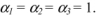
- 3) Show that α1 = α2 = α3 = 1.
Solutions
1) Basic dimensions of ϕ and of the variables
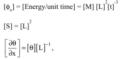
ϕ has the dimensions of a value of energy per unit time.
Therefore: ![]()
i.e.: 
or: ![]()
Moreover, the dimensions of the different variables occurring in the definition of ϕ are:

2) Maximum number of equations between parameters
Thus, the magnitude ϕ and variables λ, S and ![]() are described by four basic dimensions as follows: [M], [L], [t] and [θ].
are described by four basic dimensions as follows: [M], [L], [t] and [θ].
Therefore, according to Rayleigh’s method, the maximum number m of equations needing to be satisfied by α1, α2 and α3 is m = 4.
3) ![]()
The dimensional equation of Fourier’s law is written:

Yet:

Hence:
Thus, the following dimensional system of equations will have to be satisfied:
- – For dimension M: 1 = α1.
- – For dimension L: 2 = α1 + 2 α2 – α3.
- – For dimension T: –3 = –3 α1.
- – For dimension θ: 0 = α3 – α1.
Or, α1 = 1

i.e.: α1 = α2 = α3 = 1
4.9. Buckingham’s method
While Rayleigh’s method makes it possible to determine the number of relations existing between the exponents of the parameters involved in the expression of a given magnitude, the Buckingham π theorem, for its part, makes it possible to reduce the number of variables involved in the definition of G, grouping them into a number of dimensionless groups (Langhaar, 1951).
Indeed, let us assume that the magnitude G may be described by n variables v1, v2, …, vn:

where A is a dimensionless constant: ![]()
and let us assume that G and the values of vi are expressed as a function of m basic dimensions.
Then, according to Rayleigh’s method, there must be at most m relations between the αi values; so, the n degrees of freedom involved in the description of G in the initial equation {αi, i ∈ [1, n]} are not independent. They are linked by m relations.
Therefore, the number of parameters needed to describe G may be reduced to n-m.
Thus, Rayleigh’s method makes it possible to show that the number of parameters needed to describe variable G could be reduced to n-m independent variables.
Rayleigh’s method cannot be used to determine the independent variables concerned, however. Yet, not only do we need to determine the number of independent variables, but above all, we also need to know what these independent variables are and how each one of them is involved in the definition of G. The Buckingham π theorem, presented below, offers a step in this direction.
4.9.1. Illustration: applying the Buckingham π theorem
Consider again the example presented in section 4.8.1. The sought magnitude G is ΔP. The variables vi are seven in number; namely:
- – The flow velocity of the fluid: v.
- – The density of the fluid: ρ.
- – The viscosity of the fluid: μ.
- – The roughness of the inside walls of the pipe: ε.
- – The pipe length: l.
- – The pipe diameter: d.
- – The acceleration of gravity: g.
ΔP is written in the form:
Applying Rayleigh's method made it possible to show that the following three relations exist between the αi parameters.

Questions
- 1) By applying the Buckingham π theorem, determine the number of independent dimensionless groups that can fully describe the variable, ΔP.
- 2) Using the three relations existing between the seven αi parameters, show that ΔP can be written in the form:

- 3) Show that this relation can be written in the form:

Solutions
1) Number of independent dimensionless groups
The number m of basic dimensions involved in ΔP and in the parameters likely to be able to describe ΔP is m = 3 (see section 4.8.1 for more details).
Moreover, the number n of variables is n = 7.
By applying the Buckingham πtheorem, we obtain the number p of independent dimensionless groups describing ΔP: p = n + 1 – m.
i.e.: p = 7 + 1 – 3
2) Expression of ΔP
Yet, the following relations are satisfied by the seven αi parameters:

Hence:

Thus, by replacing α1, α2 and α6 in the expression of ΔP and by rearranging, we obtain:
3) Relation between dimensionless groups
We have:
Hence: 
Yet: 
Thus, the relation linking ΔP in a dimensionless manner to the groups of parameters conditioning it, can be written in the form:

i.e.: ![]()
4.10. Exercises and solutions
EXERCISE 4.1. Deriving the convective flux expression by dimensional analysis
We know that the flux transferred by convection between a fluid and a tube through a transfer area A with a thermal potential difference Δθ is conditioned by the following parameters:
- – The driving potential difference Δθ.
- – The transfer area A.
- – The convection heat transfer coefficient h.
In general, we will assume that:
Questions
- 1) According to Rayleigh’s method, what is the maximum number of equations that need to be satisfied by α1, α2 and α3?
- 2) Show that
Solutions
1) Maximum number of equations to be satisfied by α1, α2 and α3
- – We write:

- – The magnitude G considered is ϕ.
- – The variables are: h, A and Δθ.
According to Rayleigh's method, the maximum number of equations that need to be satisfied by α1, α2 and α3 is equal to the number of basic dimensions involved in the dimensional structures of ϕand variables h, A and Δθ.
From Table 4.2, let us determine the basic dimensions describing ϕ, h, A and Δθ.
We have:

and [Δθ] = [θ]
Thus, the magnitude considered (ϕ) and the variables (h, A and Δθ) are described by the following four base dimensions: [M], [L], [t] and [θ].
Therefore, the maximum number of equations to be satisfied by α1, α2 and α3
is four.
2) Calculating α1, α2 and α3
The dimensional equation is written: ![]()
or, alternatively, by substituting the dimensions of ϕ and of variables h, A and Δθ:
i.e.: ![]()
Hence, by grouping together the terms comprising the same dimensions:
Thus, by identifying the powers relative to each dimension, we obtain:
- – For dimension [M]: 1 = α1.
- – For dimension [L]: 2 = 2α2.
- – For dimension [t]: -3 = -3α1.
- – For dimension [θ]: 0 = α3 – α1.
Hence: α1 = 1; α2 = 1 and α3 = α1 = 1
i.e.: ![]()
EXERCISE 4.2. Expressing the radiant flux
We know that a black area S which is at a temperature T emits an energy flux depending on the following parameters:
- – the temperature T.
- – the transfer area A.
- – a constant σ, the dimensions of which are given by
In general, it will be assumed that the flux expression, as a function of these parameters, is of the form:
Questions
- 1) Based on Rayleigh's method, what is the maximum number of equations that need to be satisfied by α1, α2 and α3?
- 2) Show that α1 = α2 = 1 and that α3 = 4.
Solutions
1) Maximum number of equations to be satisfied by α1, α and α3
We have: ![]()
In this expression, the magnitude G considered is ϕ, and the variables are: σ, A and T.
According to Rayleigh's method, α1, α2 and α3 must satisfy, at most, a number of equations equal to the number of basic dimensions involved in the dimensional structures of ϕ and of variables σ, A and T.
We have: ![]()
Moreover (see Table 4.2), the dimensions describing ϕ, A and T are:

Thus, the magnitude considered (ϕ) and the variables ( σ, A and T) are described
by the four basic dimensions: [M], [L], [t] and [θ].
Therefore, the maximum number of equations that need to be satisfied by α1, α2
and α3 is four.
2) Calculating α1, α2 and α3
The dimensional equation is written: ![]()
or, alternatively, by substituting the dimensions of ϕ and of variables σ, A and T:
i.e.:
Hence, by grouping together the terms comprising the same dimensions:
Thus, by identifying the powers relative to each dimension, we obtain:
- – For dimension [M]: 1 = α1.
- – For dimension [L]: 2 = 2α2.
- – For dimension [t]: -3 = -3α1.
- – For dimension [θ]: 0 = –4α1+α3.
Hence:

i.e.: α1 = α2 = 1 and α3 = 4
EXERCISE 4.3. Driving potential difference in conductive flux
We know that the flux transferred in a solid of heat conductivity λ depends on the following parameters:
- – the area A;
- – the heat conductivity λ and
- – the driving potential difference.
We also know that the flux is given by an equation of the form:
However, we have forgotten whether, in this expression, the driving potential
difference occurs as a difference (Δθ) or as a gradient, ![]()
Questions
In order to find the correct form that needs to be used for the driving potential difference, you are asked to:
- 1) Give the dimensions of the conductive flux ϕ, the transfer area A, the heat conductivity λand the temperature difference Δθ.
- 2) Using the dimensional equation, show that the form to be used for the driving potential difference in the flux equation is differential.
Solutions
1) Dimensions of ϕ, A, λ and Δθ
These dimensions are taken from Table 4.2:

2) Form to be used for the driving potential difference in Fourier's equation
The equation giving the conductive flux is of the form:
The dimensional equation is thus: ![]()
Hence: ![]()
i.e.: ![]()
or: ![]()
that is, by simplifying: ![]()
It is therefore the dimension of a temperature by a length.
As such, it is the differential ![]() that must occur as TPD in the expression of the
that must occur as TPD in the expression of the
conductive flux, rather than Δθ.
EXERCISE 4.4. Obtaining viscosity dimensions from the Grashof number
The Grashof number is given by: 
with:
- L, the characteristic dimension of the area considered.
- ρ, the density of the fluid.
- G, the acceleration of gravity.
- β, the volumetric expansion coefficient of the constant-pressure fluid.
- ∆θ, the difference between the wall temperature and the average fluid temperature.
- μ, the viscosity of the fluid.
Question
Using dimentional analysis of this number, determine the dimensions of the viscosity μ, given that the dimension of the expansion coefficient β is the inverse of a temperature.
Solution
The dimensional equation of the Grashof number is written as follows:

Given that Gr is dimensionless, we obtain:
Yet: ![]()
and (see Table 4.2):

Hence: ![]()
That is, after simplification: ![]()
or: ![]()
EXERCISE 4.5. Dimensional analysis of the Biot number
By definition, the Biot number is given by:
where:
- h is the convective heat transfer coefficient between the liquid and the solid.
- s is a characteristic dimension of the solid considered.
- λ designates the heat conductivity of the solid considered.
Question
Based on the dimensional equation, show that Bi is indeed dimensionless.
Solution
The dimensional equation of the Biot number gives:

Yet (see Table 4.2):

and: [s] = [L]
Hence: 
Therefore, Bi is indeed dimensionless.
EXERCISE 4.6. Dimensional analysis of the Fourrier number
By definition, the Fourrier number is given by:
where:
- α is the thermal diffusivity of the material considered, defined by α = λ/ρΧπ.
- t designates the time.
- s is a characteristic dimension of the solid considered.
Question
Based on the dimensional equation, show that Fo is indeed dimensionless.
Solution
with: ![]()
We have: ![]()
i.e.: ![]()
Therefore, the dimensional equation of the Fourier number is written:

Yet (see Table 4.2):

and: [s] = [L]
Hence: 
It is therefore easy to see that Fo is indeed dimensionless.
EXERCISE 4.7. Dimensional analysis of the Froude number
By definition, the Froude number is given by: ![]()
where:
- v is the average velocity of the fluid.
- g is the acceleration of gravity.
- L is the length of the tube considered.
Question
Based on the dimensional equation, show that Fr is indeed dimensionless.
Solution
The dimensional equation relating to the Froude number gives:

Yet (see Table 4.2):


Consequently, Fr is indeed dimensionless.
EXERCISE 4.8. Dimensional analysis of the Euler number
By definition, the Euler number is given by:
where:
- ΔP is the load loss due to the flow of a fluid at velocity v.
- ρ is the density of the fluid.
- v is the average velocity of the fluid.
Question
Based on the dimensional equation, show that Eu is indeed dimensionless.
Solution
The dimensional equation relating to the Euler number gives:

Yet (see Table 4.2):

Hence: 
Therefore, Eu is indeed dimensionless.
EXERCISE 4.9. Dimensions of the expansion coefficient β
Let us recall that the Grashof number is defined by:

where:
- L is the characteristic dimension of the area considered.
- ρ is the density of the fluid.
- g is the acceleration of gravity.
- β is the volumetric expansion coefficient of the constant-pressure fluid.
- ∆ θ is the difference between the wall temperature and the average fluid temperature.
- μ is the viscosity of the fluid.
Question
Based on a dimensional analysis of the Grashof number, determine the dimensions of the expansion coefficient β.
Solution
The dimensional equation relating to the Grashof number gives:

Given that Gr is dimensionless, we obtain:
Yet (see Table 4.2):

Hence: ![]()
That is, after simplification: ![]()
EXERCISE 4.10. Dimensional analysis of the radiant flux
The flux emitted by a black area S is given by the following equation:
where σ is the Stefan–Boltzmann constant.
Questions
1) You are asked to conduct the dimensional analysis of the equation which gives the radiant flux, in order to determine the dimensions of σ.
2) Deduce the units of σ.
Solutions
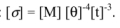
1) Dimensions of σ
The dimensional equation of the heat flux equation gives:
Hence: ![]()
Yet (see Table 4.2):

That is, by substituting in the equation which gives 
After simplification, we obtain: ![]()
2) The units of σ
We have: 
Let us analyze the different groups of dimensions appearing in the dimensional equation of [σ], making the dimensions of some standard magnitudes appear.
[M] [t]-3 recalls the dimensions of an energy flux density or a power per unit surface.
Indeed, ![]()
Hence: 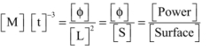
Therefore: 
σ can then be expressed in W m-2 °K-4, in kcal hr-1 m-2 °K-4, or in Btu hr-1 ft-2 °K-4.
EXERCISE 4.11. Dimensional analysis of a mass balance in a mixing tank
The mixing tank represented in Figure 4.3 is used to produce a flow rate D of sugar water, the sugar mass concentration of which must be equal to ρD.

Figure 4.3. Sweet-juice preparation tank
For this, a flow E of slightly sweet water (mass concentration ρE) is mixed with a liquid sugar concentrate C.
When the flows (E, C and D) and each of the compositions (ρE, ρC and ρD) are given in mass terms, we have demonstrated (see Exercise 1.9) that:

In this exercise, we consider that flows E and D are indeed given in mass terms (kg/hr), but flow C, on the other hand, is given in molar terms (mol/min). Likewise, concentration ρE is given in mass terms, whereas concentration ρD is given in molar terms.
Questions
1) How must equation [4.2] be modified to ensure the dimensional homogeneity of the term ![]()
2) After applying these modifications, conduct the dimensional analysis of equation [4.2].
3) Which units would you then suggest should be used for ![]() ?
?
Data:
Molar mass of liquid sugar concentrate: MC.
Solutions
1) Dimensional homogenization
The data for this problem imply the following dimensions for E, D, ρE and ρD:
- – E is given in mass terms

- – D is given in molar terms

- – ρE, ρD and ρC are fractions (mass or molar); they are therefore dimensionless.
Thus, with this dimensional data for the problem studied, we realize that it is not possible to assure dimensional homogeneity of ![]()
Indeed, as the dimensions of E and C are different, the term E + C must be modified as follows, in order to assure its dimensional homogeneity.
– Instead of E + C, we should have E + C MC, because:

– Instead of C as the numerator, we should have C MC, because:

Thus, equation [4.2] should be rewritten as follows:

2) Dimensional analysis of equation [4.2]
The dimensional equation of the first term of the equation gives:

Likewise, for the second term we obtain the following dimensions:

Yet: ![]()
Hence: 
Thus, with the modification applied to equation [4.2], the two terms of this equation will have the same dimensions. Overall dimensional homogeneity is therefore assured.
3) Units proposed
We have: 
We propose, for example: min/kg.
EXERCISE 4.12. Dimensional analysis of the mass balance of a reservoir

Figure 4.4. Feed reservoir
According to the available for D1(t) and D2(t), the differential equation governing the mass balance of the reservoir represented in figure 4.4 can be written in the following three ways:
or
where:
- S is the cross-sectional area of the reservoir.
- ρ is the density of the liquid in the tank.
- C is the molar concentration of the liquid in the tank.
- D1(t) and D2(t) are the feed and withdrawal rates. They are given by:

Of course, the form (equation [4.3], [4.4] or [4.5]) to be used for the balance equation will depend on the units of D1(t) and D2(t).
Indeed, depending on the source of the data, D1(t) and D2(t) may be available in:
- a) kg/hr.
- b) l/min or in m3/hr.
- c) mol/min.
Questions
For each of cases (a), (b) and (c) defined above:
- 1) Give the dimensions of D1(t) and D2(t).
- 2) Deduce the dimensions and units of coefficients α and β.
- 3) Based on dimensional analyses, give the form of the equation to be used depending on the case.
Solutions
1) Dimensions of D1(t) and D2(t)
- a) Case where flow rates are expressed in kg/hr:
in this case, the dimensions of D1(t) and D2(t) are: [D1] = [D2] = [M] [t]-1.
- b) Case where the flow rates are expressed in l/min or in m3/hr:
in this case, the dimensions of D1(t) and D2(t) are: [D1] = [D2] = [L]3 [t]-1.
- c) Case where flow rates are expressed in mol/min:
in this case, the dimensions of D1(t) and D2(t) are: [D1] = [D2] = [mol] [t]-1.
2) Dimensions and units of coefficients α and β
We have: D1(t) = α t2 and D2(t) = βte0,1t
2.1) Dimensions and units of α
The dimensional equation of D1(t) gives: [D1] = [α] [t]2
Hence: [α]= [D1] [t]-2
Table 4.7 gives the dimensions and units of α for each of cases (a), (b) and (c):
Table 4.7. Dimensions and units of α
| Case | Units of D1(t) | Dimensions of D1(t) | Dimensions of α | Units of α |
| (a) | kg/hr | [M] [t]-1 | [M] [t]-3 | kg/hr3 |
| (b) | l/min or m3/hr | [L]3 [t]-1 | [L]3 [t]-3 | l/min3 or (m/hr)3 |
| (c) | mol/min | [mol] [t]-1 | [mol] [t]-3 | mol/min3 |
2.2) Dimensions and units of β
The dimensional equation of D2(t) gives: [D2] = [β] [t]
Hence: [β]= [D2] [t]-1
Table 4.8 gives the dimensions and units of β for each of cases (a), (b) and (c):
Table 4.8. Dimensions and units of β
| Case | Units of D2(t) | Dimensions of D2(t) | Dimensions of β | Units of β |
| (a) | kg/hr | [M] [t]-1 | [M] [t]-2 | kg/hr2 |
| (b) | l/min or m3/hr | [L]3 [t]-1 | [L]3 [t]-2 | l/min2 or m3/hr2 |
| (c) | mol/min | [mol] [t]-1 | [mol] [t]-2 | mol/min2 |
3) Form of the equation to be used depending on the case
The three forms are as follows:
– Form (1): ![]()
– Form (2): ![]()
– Form (3): 
The form of the equation to be used will depend on the first member of each of these equations. Dimensional analysis of the first side of each of the forms gives the following results:
– For form (1):

– For form (2):

– For form (3):

Dimensional homogeneity requires these dimensions to be those of D1(t) and D2(t).
For each of cases (a), (b) and (c), Table 4.9 gives the dimensions of D1 and D2, as well as the form of the equation to be used:
Table 4.9. Dimensions of D1 and D2
| Case | Dimensions of D2(t) and D2(t) | Form to be used |
| (a) | [M] [t]-1 | 2 |
| (b) | [L]3 [t]-1 | 1 |
| (c) | [mol] [t]-1 | 3 |
EXERCISE 4.13. Dimensional analysis of the heat balance of a calorimeter
Using the heat balance of a calorimeter, it is possible to link the amount of heat Q that the calorimeter transfers to the fluid, to the increase in temperature (from T1 to T2) of the fluid through the following equation:
Where M is the mass of the fluid in the calorimeter and Cp is its heat capacity.
Questions
- 1) What are the dimensions of Q?
- 2) From the dimensional equation, determine the dimensions of Cp.
- 3) Deduce the units of Cp, according to the International System.
- 4) Q is given in kW-hour, M in kg and T in °C: what should the units of Cp then be?
Solutions
1) Dimensions of Q
Q is an energy value. Therefore, its dimensions are (see Table 4.2):
2) Dimensions of Cp
The dimensional equation of the heat balance gives:
Hence: ![]()
or: ![]()
i.e.: ![]()
3) Units of Cp in the International system
We have: ![]()
Yet, [L] 2 [t]-2 is the dimension of an energy per unit mass:

Consequently: 
Hence: 
In the International System:

Consequently, the units of Cp in the IS are: 
4) Units of Cp if Q was in kW-hour

In the present case, we have:

EXERCISE 4.14. Dimensional analysis of the Lennard–Jones potential
The Lennard–Jones potential is used to model the interactions of molecules with one another, rather like in a gravitational field. The potential field ϕ specific to these interactions is given by:

where:
- r is the distance between centers of molecules
- ε is the energy that characterizes the interaction between molecules
- σ is the characteristic diameter of the molecule, also called the collision diameter
Questions
- 1) Give the dimensions of r, ε and σ.
- 2) Deduce the dimensions of φ(r).
- 3) In this model, the interaction force between two molecules, A and B, is expressed as a function of the potential gradient:
 . Give the dimensions of FAB.
Solutions
1) Dimensions of r, ε and σ

2) Dimensions of φ(r)

![]() is dimensionless, therefore:
is dimensionless, therefore: ![]()
Thus: ![]()
3) Dimensions of FAB
We have: ![]()
Therefore: ![]()
Yet: ![]()
i.e.: ![]()
or: ![]()
EXERCISE 4.15. Dimensions and units of the Planck constant
We know that a photon carries an amount of energy E which depends on the wavelength λ(or on the frequency ν) of the radiation according to the relation:
h is the Planck constant.
c is the speed of light.
Questions
- 1) Give the dimensions of E, c and λ.
- 2) Deduce the dimensions of h.
- 3) Propose units for h in a coherent system.
Solutions
1) Dimensions of E, c and λ

2) Dimensions of h
We have: ![]()
Therefore: 
Hence: 
Thus: 
i.e.: ![]()
3) Units for h
We know that [M] [L] 2 [t]-2 is the dimension of an energy.
Thus, in the International System, h will be expressed in Joules × seconds;
i.e.: ![]()
EXERCISE 4.16. Dimensional analysis of the heat balance of a water heater
An electric water heater of volume V permits the heating of a flow rate D of water from T1 to T2. The heat balance of this heater is given by:
where:


- P is the electrical power of the water heater;
- η is a heating efficiency coefficient;
- V is the volume of the water heater and
- ρ is the density of the water and Cp its sensible heat.
Questions
1) Without using the dimensions of parameters D, ρ, V, η, P and Cp, which define groups αand β, what are the dimensions of these groups?
2) Using the fact that ![]() , deduce that ηis dimensionless.
, deduce that ηis dimensionless.
Solutions
1) Dimensions of groups α and β
Dimensional analysis of the differential equation gives:
and:

Hence: 
and: ![]()
2) Dimensions of η
We have: 
Hence: 
Yet: 

Hence:

Therefore, η is indeed dimensionless.
EXERCISE 4.17. Dimensions of the perfect gas constant
The osmotic pressure πof a solution depends on temperature concentration as follows:

where:
- T is the absolute temperature;
- R is the perfect gas constant;
- V is the volume and a is the solution activity.
Questions
- 1) Give the dimensions of V, T and π.
- 2) Deduce the dimensions of R.
- 3) Propose units for R in a coherent system.
Solutions
1) Dimensions of V, T and π

2) Dimensions of R
Thus: ![]()
That is, by substituting for [π], [V] and [T]:
i.e.: ![]()
3) Units for R

[M] [L] 2 [t]-2 is the dimensional structure of an energy.

Thus, R may be expressed in J/°C, in cal/°C, in Btu/°F, etc.
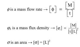
EXERCISE 4.18. Dimensions of the osmosis coefficient
During the balancing by osmosis of the concentrations, C1 and C2, of two compartments, the osmotic flux density is expressed as follows:
φ is the molar density of the osmotic flux.
C1 and C2 are the solute molar concentrations in compartments 1 and 2, respectively.
E is the thickness of the semi-permeable membrane.
D is the solute diffusion coefficient through osmosis; this data is provided by the manufacturer of the semipermeable membrane.
Questions
- 1) Give the dimensions of φ, C and E.
- 2) Deduce the dimensions of D.
- 3) Propose units for D in a coherent system.
Solutions
1) Dimensions of φ, C and E
- φ is a density of the molar flux → [φ] = [mol] [t]-1 [L]-2
- C is a molar concentration → [C] = [mol] [L] -3
- E is a thickness → [E] = [L]
2) Dimensions of D
Hence:
That is, by substituting the dimensions of φ, C and E:

i.e.: ![]()
3) Units for D
cm2/sec, m2/min, in2/sec, etc.
EXERCISE 4.19. Dimensions of a heat balance equation

Figure 4.5. Stirred tank with a steam jacket
The stirring and heating tank presented in Figure 4.5 enables sweet juice to be produced by mixing a flow d of sugar syrup with a flow D of pure water.
In order to accelerate dissolution, the tank is stirred with a propeller mixer and heated by steam.
The heat balance in steady state is written as follows:
The different parameters are defined in the technical data sheet presented in Table 4.10.
Table 4.10. Technical data sheet
| Variable | Designation |
| D | Mass flow of water at input, temperature T0 |
| J | Mass flow of sweet water produced, temperature T |
| d | Mass flow of sugar syrup |
| Cpd | Sensible heat of d |
| CpD | Sensible heat of D |
| CpJ | Sensible heat of J |
| V | Mass flow of steam |
| Λ | Latent heat of condensation of the saturated steam |
| Q | Flux of heat losses |
Questions
- 1) Give the dimensions of Q, V, D and J and of the sensible heats.
- 2) Based on a dimensional analysis of the energy balance equation, determine the dimensions of the latent heat of condensation of the saturated steam.
- 3) Propose coherent units for this parameter.
Solutions
1) Dimensions of Q, V, D and J and of the sensible heats

i.e.: ![]()
V, D, d and J are mass flow rates → [V] = [M] [t]-1

The sensitive heat values have the dimensions of an energy per unit mass and per unit temperature.
i.e.: 
or ![]()
2) Dimensions of Λ
The heat balance equation is written as:
Dimensional homogeneity implies: [V Λ] = [Q]

3) Units of Λ
We have: [Λ] = [L]2 [t]-2
We know that [M] [L] 2 [t]-2 is the dimensional structure of an energy.
Therefore, [L] 2 [t]-2 is the dimensional structure of an energy per unit mass.

As a result, Λ may be expressed in J/g, in cal/kg, in Btu/lb, etc.
EXERCISE 4.20. Homogeneity of the reverse-osmosis sizing equation
In a multi-stage reverse-osmosis system (see Figure 4.6), the total number N of modules needed to perform a given desalination operation is linked to the mass flow rate ϕ to be treated by:

where:
- ϕ is the total mass flow rate;
the flow rate treated by each module is then:

- η is the number of stages in the system;
- m is the number of reverse-osmosis modules per stage;
- φs is the mass flux density that can be reached by a module;
- σ is the transfer area of a cell: manufacturer's data.

Figure 4.6. Staged reverse-osmosis unit
Questions
- 1) Give the dimensions of ϕ, φS and σ.
- 2) Verify, as a consequence, the dimensional homogeneity of this relation.
Solutions
1) Dimensions of φ, ϕS and σ
2) Verifying the dimensional homogeneity
We have: 
Because N is dimensionless, homogeneity will require:
With n being dimensionless, we need to have:
This is satisfied because:

EXERCISE 4.21. Permeability dimensions of a reverse-osmosis membrane
During a reverse-osmosis purification operation, the flux density of the solvent passing through the semipermeable membrane, under the action of a pressure gradient ΔP, is given by:
where:
- φS is the mass flux density of the solvent passing through the semi-permeable membrane;
- ψS is the membrane's permeability to the solvent;
- ΔP is the difference in pressure between the two compartments;
- E is the thickness of the membrane.
Questions
- 1) Give the dimensions of φS, ΔP and E.
- 2) Deduce the dimensions of ψS.
- 3) Propose units for ψS in a coherent system.
Solutions
1) Dimensions of φS , ΔP and E
φS is a mass flux density ![]()
ΔP has the dimensions of a pressure value ![]()
E is a thickness → [E] = [L]
2) Dimensions of ψΣ
We have: ![]()
Hence: ![]()
That is, by substituting in the dimensions of φΣ, ΔP and E:
or: ![]()
3) Units for ψS
or: ![]()
or: ![]() , etc.
, etc.
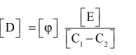
EXERCISE 4.22. Dimensions of the overall dialysis coefficient
The flux of a solute passing through the membrane of a dialyzer is given by the following equation (Lane & Riggle, 1959):
where:
- ϕ is the mass flux of the solute passing through the membrane.
- U is the overall dialysis coefficient.
- C is data provided by the membrane manufacturer.
- A is the transfer area: membrane area.
- ΔCmL is the logarithmic mean of the difference in concentration between the two sides of the membrane:

Questions
- 1) Give the dimensions of ϕ, ΔCmL and A.
- 2) Deduce the dimensions of the overall dialysis coefficient U.
- 3) Propose units for U in a coherent system.
Solutions
1) Dimensions of ϕ, ΔCmL and A
ΔCmL has the dimensions of a mass concentration.
Indeed: 
Hence: ![]()
i.e.: ![]()
A is an area → [A] = [L]2
2) Dimensions of the overall dialysis coefficient U
The overall dialysis coefficient is linked to the mass flux by:
Hence: ![]()
That is, by substituting the dimensions: ![]()
i.e.: ![]()
3) Units for U
U can therefore be expressed in cm/s, in ft/min, etc.
EXERCISE 4.23. Permeability dimensions of a dialysis membrane
In dialysis, an important parameter is the permeability Um of the membrane to the solute. The following empirical relation links this parameter to the diffusion coefficient D of this solute through the membrane (dimensions: [D] = [L]2 [t]-1):
where:
- F is a non-dimensional factor.
- ε is the volume fraction of the membrane occupied by the pores.
- h is the tortuosity, defined as the ratio between the capillary length of the pores and the membrane thickness.
- z is the wet thickness of the membrane.
Question
What are the dimensions of Um?
Solution
Um is given by: ![]()
Hence: ![]()
As F, ε and h are dimensionless, then: ![]()
Hence: ![]()
i.e.: ![]()
EXERCISE 4.24. Dimensions of the separation capacity of a centrifuge
The separation capacity, ΔUmax, of a Zippe centrifuge is expressed as a function of its peripheral velocity V as follows:

where:
- Z is the centrifuge height;
- C is the molar concentration;
- D is the diffusion coefficient (dimensions: [D ] = [L]2 [t]-1);
- ΔM is the difference between the molar masses of the two molecules to be separated;
- V is the peripheral velocity of the centrifuge;
- T is the absolute temperature;
- R is the perfect gas constant.
Questions
- 1) Give the dimensions of C, ΔM, V and R.
- 2) What are the dimensions of the ratio:

- 3) Deduce the dimensions of the separation capacity ΔU.
- 4) Propose units for U in a coherent system.
Solutions
1) Dimensions of C, ΔM, V and R
C is a molar concentration ![]()
ΔM has the dimensions of a molar mass ![]()
V is a velocity ![]()
By definition, R is given by: 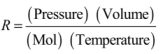
and: [Pressure] = [M] [L]-1 [t]-2
Hence: 
Therefore: ![]()
2) Dimensions of the ratio 
The dimensional equation is thus: 
i.e. by substituting the dimensions of the different magnitudes:

χ is then dimensionless.
3) Dimensions of the overall dialysis coefficient U
We have ![]()
Hence: ![]()
or: ![]()
That is, by replacing by the dimensions: ![]()
That is, ultimately: ![]()
4) Units of U:
U can then be expressed in mol/sec.
EXERCISE 4.25. Dimensions of flux transferred by electrodialysis
In an electrodialysis unit, the flux density of the mass transferred depends on the electric field imposed at the cell terminals. The relation that reflects this dependency is not dimensionless. It gives the max flux density as a function of the parameters of the problem:
where:
- zi is the valence of the ion considered;
- v is the average velocity (cm/s);
- ∇E is the electric field gradient (volts/cm);
- F is the Faraday constant (C/g);
- ci is the concentration of i (g/cm3);
- λι is the ion conductance (cm2/Ω g);
- ui is the ion mobility of i:

Questions
- 1) Give the dimensions of φι, v, ∇E, zi, F and ci.
- 2) Show that dimensional homogeneity results in:

- 3) Deduce the dimensions of λι.
- 4) What dimensions of Di would enable dimensional homogeneity to be assured for the equation giving φι?
- 5) As a function of the units proposed for the different parameters, which units would you suggest retaining for φι?
Solutions
1) Dimensions of φι, v, ∇ Ε, zi, F and ci.

Yet (see Table 4.2): [E] = [M] [L]2 [t]-3 [I]-1
Hence: [∇E] = [M] [L] [t]-3 [I]-1

2) Dimensions of u1
Dimensional homogeneity results in: ![]()
Hence: ![]()
3) Dimensions of λi
We have: ![]()
The dimensional equation of this expression of ui gives: ![]()
or, alternatively, by replacing [ui] with ![]()
Hence: ![]()
That is, by substituting the dimensions of [φι], [F], [ci] and [∇E]:
That is, after simplification: ![]()

i.e.: 
λi is the ion conductance → [λι] = [Area] [Electrical resistance]-1[M] -1
Yet: [Electrical resistance] = [M] [L]2 [t]-3 [I]-2
Hence: ![]()
i.e.: ![]()
4) Dimensions of Di
Dimensional homogeneity results in: ![]()
Hence:

i.e.: ![]()
or: ![]()
5) Units of φi
We have: ![]()
The units of φiwill be those of the term civ:

Hence: <φi> = g/cm3sec.
EXERCISE 4.26. Dimensions of electrodialysis power consumption
The power consumption of an electrodialyzer is given by the equation:

with:
- E, the average specific consumption (kWh/m3);
- F, the water volumetric flow rate (m3/hr);
- Re, the electrical resistance of a cell of the electrolyzer (ohms);
- Ae, the active area of the membrane of a cell of the electrolyzer (m2);
- U, the voltage applied to the terminals of an electrolysis cell (volts);
- n, the number of cells.
Questions
- 1) Determine the dimensions of E.
- 2) As a function of the units given below, what units of E would result from the equation?
Data:
Solutions
1) Dimensions of E


Yet:
- F is a volumetric flow rate → [F] = [L]3 [t]-1
- Re is an electrical resistance → [Re] = [M] [L]2 [t]-3 [I]-2
- Ae is an area → [Ae] = [L]2
- U is an electric potential difference → [U] = [M] [L]2 [t]-3 [I]-1
Hence: 
or: ![]()
i.e.: ![]()
2) Units of E
We know that [M] [L] 2 [t]-2 is the dimensional structure of an energy.
Thus: ![]()
Therefore: ![]()
4.11. Reading: Osborne Reynolds and Ludwig Prandtl
4.11.1. Osborne Reynolds
Renowned Irish physicist Osborne Reynolds was born on August 23, 1842 in Belfast (Northern Ireland).
With a background in engineering, Reynolds made important contributions that helped to structure fluid dynamics theory.

(source: https://fr.wikipedia.org/wiki/Fichier:OsborneReynolds.jpg)
He is thus considered to be one of the founders of fluid mechanics, thanks to his many contributions to hydrodynamics in general, and to fluid dynamics in particular.
His most significant contribution to the study of fluids in motion was the establishment of a methodology to characterize a fluid's motion through the calculation of a dimensionless number. This number, which as we know is of great importance to the practice of fluid engineering, came to be known as the Reynolds number.
Indeed, it was Reynolds who, in 1883, first proposed using this number to determine whether water flow will occur in parallel (laminar) layers or rather in a sinuous manner (turbulent). This theoretical development, tried and tested through experimentation, appeared in January 1883 in his article entitled “An Experimental Investigation of the Circumstances Which Determine Whether the Motion of Water Shall Be Direct or Sinuous, and of the Law of Resistance in Parallel Channels”, published in Philosophical Transactions, volume 174 (Royal Society of London).
As well as being a brilliant researcher, Osborne Reynolds also taught engineering. He was among those who argued that all engineering students should have a solid foundation of knowledge in mathematics and physics. Despite his great interest in teaching he was not, however, a great teacher! In the opinion of his former students, his classes were complicated and hard to follow. He had difficulty simplifying the knowledge he had to convey: a great scientist but a poor educator, often changing subject during a presentation without taking care to ensure the necessary connections and transitions.
Nevertheless, and thanks above all to his brilliant contributions to the field of research, he became the holder of one of only two engineering chairs existing at that time. He directed the chair of the unit, which later became the University of Victoria in Manchester. He died on February 21, 1912 in Watchet (England).
4.11.2 Ludwig Prandtl
When characterizing Ludwig Prandtl, one would be quick to describe him as a highly-valued scientist.
His training was both conventional and solid. After obtaining a degree in physics from Ludwig-Maximilian University in Munich, he began studying for a postgraduate degree in engineering at the same university.

(source: https://fr.wikipedia.org/wiki/Fichier:Prandtl_portrait.jpg)
His dissertation, presented on November 14, 1899, entitled Lateral Displacement Phenomena, a Case of Unstable Equilibrium, dealt with the stability of combustion equilibria. He continued his research at the same university, where he obtained the title of Doctor of Science.
He began his working life developing assembly lines for MAN factories. Here, the realities on the ground first led him to develop an interest in fluid mechanics. Indeed, it was as a result of analyzing the operating mode of a dust collector that he came to explore the fundamentals and explanations that could lead to potential improvements in performance.
He taught at the University of Hanover (Gottfried-Wilhelm Leibnitz University) and at the University of Göttingen where, betwee en 1906 and 1908, he supervised the research work of the young Theodore von Kármán with the goal of obtaining his doctorate.
Ludwig Prandtl's contributions to boundary layer theory, which he had introduced in 1904, offered him unchallenged leadership in the field. He was appointed director of the brand-new Max Planck Institute for Fluid Dynamics in Göttingen in 1909.
Starting in 1907, he focused on supersonic flows and the shock waves that must accompany them.
The prospects that opened up as a result of nascent aerodynamics and aeronautics applications gave great importance to his work. He then developed a method for visualizing the oscillations of air layers at the outlet of a de Laval nozzle and in 1908, he oversaw the construction of Germany's first wind tunnel.
In 1910, he was the first to introduce a dimensionless number into the description of turbulent flows. This number came to be called the Prandtl number.
Analysis of supersonic flows and the experimental installations at his disposal allowed him to then develop his theory of airfoils, which would come to form the basis of aerodynamics and modern aeronautical engineering. Thus, he developed an acceptable formula for the calculation of lift, and developed, back in 1919, a drag theory enabling the design and calculation of aircraft wing profiles. In 1929, he developed a reactor calculation method that continues to be used in missile design.
Four major achievements of this great man of science are to be remembered in particular, since they remain to this day of great use in engineering calculations and in aerodynamic technologies:
- 1) Boundary layer theory, which makes it possible to explain several manifestations of mass diffusion heat transfer.
- 2) The dimensionless number, which he introduced in 1910 to describe turbulent flows. This number, which subsequently became known as the Prandtl number, continues to be used in transfer calculations.
- 3) His work on hydraulics, published in 1931 under the title Führer durch die Strömungslehre.
- 4) The probe he developed for determining the relative velocity of an object in an aerodynamic environment. This is the Prandtl probe.
Prandtl's work published in 1931 can be considered as the ultimate reference for studies on laminar and turbulent flow, boundary layer, fluid mechanics, supersonic flows and the shock waves that must accompany them, as well as aerodynamics and aeronautical applications. This work also serves as a reference in the field of visualization of air-layer oscillations at the outlet of a nozzle.
The Prandtl probe, a variant of the Pitot tube, continues to be used in aerodynamics to this day: using this probe we are at present able to appreciate an aircraft’s velocity in relation to the wind.