CHAPTER 14

More Network Algorithms

Chapter 13 focused on network traversal algorithms, including algorithms that use breadth-first and depth-first traversals to find the shortest paths between nodes in the network. This chapter continues the discussion of network algorithms. The first algorithms, which perform topological sorting and cycle detection, are relatively simple. The algorithms described later in the chapter, such as graph coloring and maximal flow calculation, are a bit more complicated.

Topological Sorting

Suppose you want to perform a complicated job that involves many tasks, some of which must be performed before others. For example, suppose you want to remodel your kitchen. Before you can get started, you may need to obtain permits from your local government. Then you need to order new appliances. Before you can install the appliances, however, you need to make any necessary changes to the kitchen's wiring. That may require demolishing the walls, changing the wiring, and then rebuilding the walls. A complex project such as remodeling an entire house or commercial building might involve hundreds of steps with a complicated set of dependencies.

Table 14-1 shows some of the dependencies you might have while remodeling a kitchen.

Table 14-1: Kitchen Remodeling Task Dependencies

TASK	PREREQUISITE
Obtain permit	—
Buy appliances	—
Install appliances	Buy appliances
Demolition	Obtain permit
Wiring	Demolition
Drywall	Wiring
Plumbing	Demolition
Initial inspection	Wiring
Initial inspection	Plumbing
Drywall	Plumbing
Drywall	Initial inspection
Paint walls	Drywall
Paint ceiling	Drywall
Install flooring	Paint walls
Install flooring	Paint ceiling
Final inspection	Install flooring
Tile backsplash	Drywall
Install lights	Paint ceiling
Final inspection	Install lights
Install cabinets	Install flooring
Final inspection	Install cabinets
Install countertop	Install cabinets
Final inspection	Install countertop
Install flooring	Drywall
Install appliances	Install flooring
Final inspection	Install appliances

You can represent the job's tasks as a network in which a link points from task A to task B if task B must be performed before task A. Figure 14-1 shows a network that represents the tasks listed in Table 14-1.

A partial ordering is a set of dependencies that defines an ordering relationship for some but not necessarily all the objects in a set. The dependencies listed in Table 14-1 and shown in Figure 14-1 define a partial ordering for the remodeling tasks.

Figure 14-1: You can represent a series of partially ordered tasks as a network.

If you want to actually perform the tasks, you need to extend the partial ordering to a complete ordering so that you can perform the tasks in a valid order. For example, the conditions listed in Table 14-1 don't explicitly prohibit you from installing the flooring before you do the plumbing work, but if you carefully study the table or the network, you'll see that you can't do those tasks in that order. (The flooring must come after painting the walls, which must come after drywall, which must come after plumbing.)

Topological sorting is the process of extending a partial ordering to a full ordering on a network.

One algorithm for extending a partial ordering is quite simple. If the tasks can be completed in a valid order, there must be some task with no prerequisites that you can perform first. Find that task, add it to the extended ordering, and remove it from the network. Then repeat those steps, finding another task with no prerequisites, adding it to the extended ordering, and removing it from the network until all the tasks have been completed.

If you reach a point where every remaining task has a prerequisite, then the tasks have a circular dependency so the partial ordering cannot be extended to a full ordering.

The following pseudocode shows the basic algorithm:

The basic idea behind the algorithm is straightforward. The trick is implementing the algorithm efficiently. If you just look through the network at each step to find a task with no prerequisites, you might perform O(N) steps each time, for a total run time of O(N²).

A better approach is to give each network node a new NumBeforeMe property that holds the number of a node's prerequisites and initialize each node's NumBeforeMe value. Now when you remove a node from the network, follow its links and decrement the NumBeforeMe property for the nodes that are dependent on the removed node. If a node's NumBeforeMe count becomes 0, it is ready to add to the extended ordering.

The following pseudocode shows the improved algorithm:

This algorithm assumes that the network is completely connected. If it is not, use the algorithm repeatedly for each connected component.

Cycle Detection

Cycle detection is the process of determining whether a network contains a cycle. In other words, it is the process of determining whether a path through the network returns to its beginning.

Cycle detection is easy if you think of the problem as one of topological sorting. A network contains a cycle if and only if it cannot be topologically sorted. In other words, if you think of the network as a topological sorting problem, the network contains a cycle if a series of tasks A, B, C, ..., K forms a dependency loop.

After you make that observation, detecting cycles is easy. The following pseudocode shows the algorithm:

This algorithm assumes that the network is completely connected. If it is not, use the algorithm repeatedly for each connected component.

Map Coloring

In map coloring, the goal is to color the regions in a map so that no regions that share an edge have the same color. Obviously you can do this if you give every region a different color. The real question is, “What is the smallest number of colors you can use to color a particular map?” A related question is, “What is the smallest number of colors you can use to color any map?”

To study map coloring with network algorithms, you need to convert the problem from one of coloring regions into one of coloring nodes. Simply create a node for each region, and make an undirected link between two nodes if their corresponding regions share a border.

Depending on the map, you may be able to color it with two, three, or four colors. The following sections describe these maps and algorithms you can use to color them.

Two-coloring

Some maps, such as the one shown in Figure 14-2, can be colored with only two colors.

Figure 14-2: Some maps can be colored with only two colors.

Coloring this kind of map is easy. Pick any region, and give it one of the two colors. Then give each of its neighbors the other color, and recursively visit them to color their neighbors. If you ever come to a point where a node's neighbor already has the same color as the node, the map cannot be two-colored.

The following pseudocode shows this algorithm:

This algorithm assumes that the network is completely connected. If it is not, use the algorithm repeatedly for each connected component.

Three-coloring

It turns out that determining whether a map is three-colorable is a very difficult problem. In fact, no known algorithm can solve this problem in polynomial time.

One fairly obvious approach is to try each of the three colors for the nodes and see if any combination works. If the network holds N nodes, this takes O(3^N) time, which is quite slow if N is large. You can use a tree traversal algorithm, such as one of the decision tree algorithms described in Chapter 12, to try combinations, but this still will be a very slow search.

You may be able to improve the search by simplifying the network. If a node has fewer than three neighbors, those neighbors can use at most two of the available colors, so the original node can use one of the unused colors. In that case, you can remove the node with fewer than three neighbors from the network, color the smaller network, and then restore the removed node, giving it a color that isn't used by a neighbor.

Removing a node from the network reduces the number of neighbors for the remaining nodes, so you might be able to remove even more nodes. If you're lucky, the network will shrink until you're left with a single node. You can then color that node and add the other nodes back into the network, coloring each in turn.

The following steps describe an algorithm that uses this approach:

1. Repeat while the network has a node with degree less than 3:
   1. Remove a node with degree less than 3, keeping track of where the node was so that you can restore it later.
2. Use a network traversal algorithm to find a three-coloring for whatever network remains. If there is no solution for the smaller network, there is no solution for the original network.
3. Restore the nodes removed earlier in last-removed-first-restored order, and color them using colors that are not already used by their neighbors.

If the network is not completely connected, you can use the algorithm for each of its connected components.

Four-coloring

The four-coloring theorem states that any map can be colored with at most four colors. This theorem was first proposed by Francis Guthrie in 1852 and was studied extensively for 124 years before Kenneth Appel and Wolfgang Haken finally proved it in 1976. Unfortunately, their proof exhaustively examined a set of 1,936 specially selected maps, so it doesn't offer a good method of finding a four-coloring of a map.

You can use techniques similar to those described in the previous section for three-coloring.

1. Repeat while the network has a node with degree less than 4:
   1. Remove a node with degree less than 4, keeping track of where the node was so that you can restore it later.
2. Use a network traversal algorithm to find a four-coloring for whatever network remains. If there is no solution for the smaller network, there is no solution for the original network.
3. Restore the nodes removed earlier in last-removed-first-restored order, and color them using colors that are not already used by their neighbors.

Again, if the network is not completely connected, you can use the algorithm for each of its connected components.

Five-coloring

Even though no simple constructive algorithm exists for four-coloring a map, there is one for five-coloring, even if it isn't very simple.

Like the algorithms described in the two previous sections, this algorithm repeatedly simplifies the network. Unlike the two previous algorithms, this one can always simplify the network until it eventually contains only a single node. You can then undo the simplifications to rebuild the original network, coloring the nodes as you do.

This algorithm uses two types of simplification. The first is similar to the one used by the two previous algorithms. If the network contains a node that has fewer than five neighbors, remove it from the network. When you restore the node, give it a color that is not used by one of its neighbors. Call this Rule 1.

You use the second simplification if the network doesn't contain any node with fewer than five neighbors. It can be shown (although it's outside the scope of this book) that such a network must have at least one node K with neighbors M and N such that:

• K has exactly five neighbors.
• M and N have at most seven neighbors.
• M and N are not neighbors of each other.

To simplify the network, find such nodes K, N, and M, and require that nodes M and N have the same color. We know that they aren't neighbors, so that is allowed. Because node K has exactly five neighbors and nodes M and N use the same color, K's neighbors cannot be using all five of the available colors. That means at least one is left over for node K to use.

The simplification is to remove nodes K, M, and N from the network and create a new node M/N to represent the color that nodes M and N will have. Give the new node the same neighbors that nodes M and N had previously. Call this Rule 2.

When you restore the nodes K, M, and N that were removed using Rule 2, give nodes M and N whatever color was assigned to node M/N. Then pick a color that isn't used by one of its neighbors for node K.

You can use techniques similar to those described in the previous section for three-coloring. The following steps describe the algorithm:

1. Repeat while the network has more than one node:
   1. If there is a node with degree less than 5, remove it from the network, keeping track of where it was so that you can restore it later.
   2. If the network contains no node of degree less than 5, find a node K with degree exactly 5 and two children M and N, as described earlier. Remove nodes K, M, and N, and create the new node M/N as described in Rule 1.
2. When the network contains a single node, assign it a color.
3. Restore the previously removed nodes, coloring them appropriately.

If the network is not completely connected, you can use the algorithm for each of its connected components.

Figure 14-4 shows a small sample network being simplified. If you look closely at the network at the top, you'll see that every node has five neighbors, so you can't use Rule 1 to simplify the network.

Although you cannot use Rule 1 on this network, you can use Rule 2. There are several possible choices for nodes to play the roles of nodes K, M, and N in Rule 2. This example uses the nodes C, B, and H. Those nodes are removed, and a new node B/H is added with the same children that nodes B and H had before.

After nodes C, B, and H have been replaced with the new node B/H, nodes G, A, and D have fewer than five neighbors, so they are removed. (For this example, assume that they are removed in that order.)

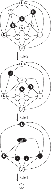
Figure 14-4: You can simplify this network to a single node with one use of Rule 2 and several uses of Rule 1.

After those nodes have been removed, nodes L, B/H, K, F, E, and I all have fewer than five neighbors, so they are removed also.

At that point the network contains only the single node J, so the algorithm arbitrarily assigns node J a color and begins reassembling the network.

Suppose the algorithm gives nodes the colors red, green, blue, yellow, and orange, in that order. For example, if a node's neighbors are red, green, and orange, the algorithm gives the node the first unused color—in this case, blue.

Starting at the final network shown in Figure 14-4, the algorithm follows these steps:

1. The algorithm makes node J red.
2. The algorithm restores the node that was removed last, node I. Node I's neighbor J is red, so the algorithm makes node I green.
3. The algorithm restores the node that was removed next-to-last, node E. Node E's neighbors J and I are red and green, so the algorithm makes node E blue.
4. The algorithm restores node F. Node F's neighbors J and E are red and blue, so the algorithm makes node F green.
5. The algorithm restores node K. Node K's neighbors J and F are red and green, so the algorithm makes node K blue.
6. The algorithm restores node B/H. Node B/H's neighbors K, F, and I are blue, green, and green, so the algorithm makes node B/H red.
7. The algorithm restores node L. Node L's neighbors K, B/H, and I are blue, red, and green, so the algorithm makes node L yellow. (At this point the network looks like the bottom network in Figure 14-4, but with the nodes colored.)
8. The algorithm restores node D. Node D's neighbors B/H, E, and I are red, blue, and green, so the algorithm makes node D yellow.
9. The algorithm restores node A. Node A's neighbors B/H, F, E, and D are red, green, blue, and yellow, so the algorithm makes node A orange.
10. The algorithm restores node G. Node G's neighbors L, B/H, and K are yellow, red, and blue, so the algorithm makes node G green. (At this point the network looks like the middle network in Figure 14-4, but with the nodes colored.)
11. Now the algorithm undoes the Rule 2 step. It restores nodes B and H and gives them the same color as node B/H, which is red. Finally, it restores node C. Its neighbors G, H, D, A, and B have colors green, red, yellow, orange, and red, so the algorithm makes node C blue. (At this point the network looks like the network at the top of Figure 14-4, but with the nodes colored.)

Figure 14-5 shows the original network. Nodes of different colors are represented by different shapes because this book is black and white.

Figure 14-5: Shapes show nodes of different colors in this five-colored network.

Other Map-coloring Algorithms

These are not the only possible map-coloring algorithms. For example, a hill-climbing strategy might loop through the network's nodes and give each one the first color that is not already used by one of its neighbors. This may not always color the network with the fewest possible colors, but it is extremely simple and very fast. It also works if the network is not planar and it might be impossible to four-color the network. For example, this algorithm can color the non-planar network shown in Figure 14-6.

Figure 14-6: This network is not planar but can be three-colored.

With some effort, you could apply some of the other heuristic techniques described in Chapter 12 to try to find the smallest number of colors needed to color a particular planar or nonplanar network. For example, you could try random assignments or incremental improvement strategies in which you switch the colors of two or more nodes.

Maximal Flow

In a capacitated network, each of the links has a maximum capacity indicating the maximum amount of some sort of flow that can cross it. The capacity might indicate the number of gallons per minute that can flow through a pipe, the number of cars that can move through a street per hour, or the maximum amount of current a wire can carry.

In the maximal flow problem, the goal is to assign flows to the links to maximize the total flow from a designated source node to a designated sink node.

For example, consider the networks shown in Figure 14-7. The numbers on a link show the link's flow and capacity. For example, the link between nodes B and C in the left network has a flow of 1 and a capacity of 2.

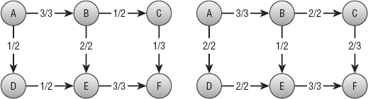
Figure 14-7: In the maximal flow problem, the goal is to maximize the flow from a source node to a sink node.

The network on the left has a total flow of 4 from node A to node F. The total amount of flow leaving the source node A in the network on the left is 1 unit along the A → D link plus 3 units along the A → B link for a total of 4. Similarly the total flow into the sink node F is 3 units along the E → F link plus 1 unit along the C → F link for a total of 4 units. (If no flow is gained or lost in the network, then the total flow out of the sink node is the same as the total flow into the sink node.)

You cannot increase the total flow by simply adding more flow to some of the links. In this example you can't add more flow to the A → B link because that link is already used at full capacity. You also can't add more flow to the A → D link because the E → F link is already used at full capacity, so the extra flow wouldn't have anywhere to go.

You can improve the solution, however, by removing 1 unit of flow from the path B → E → F and moving it to the path B → C → F. That gives the E → F link unused capacity so you can add a new unit of flow along the path A → D → E → F. The network on the right in Figure 14-7 shows the new flows, giving a total flow of 5 from node A to node F.

The algorithm for finding maximal flows is fairly simple, at least at a high level, but figuring out how it works can be hard. To understand the algorithm, it helps to know a bit about residual capacities, residual capacity networks, and augmenting paths.

If that sounds intimidating, don't worry. These concepts are useful for understanding the algorithm, but you don't need to build many new networks to calculate maximal flows. Residual capacities, residual capacity networks, and augmenting paths can all be found within the original network without too much extra work.

A link's residual capacity is the amount of extra flow you could add to the link. For example, the C→ F link on the left in Figure 14-7 has a residual capacity of 2 because the link has a capacity of 3 and is currently carrying a flow of only 1.

In addition to the network's normal links, each link defines a virtual backlink that may not actually be part of the network. For example, in Figure 14-7 the A → B link implicitly defines a backwards B → A backlink. These backlinks are important because they can have residual capacities, and you may be able to push flow backwards across them.

A backlink's residual capacity is the amount of flow traveling forward across the corresponding normal link. For example, on the left in Figure 14-7 the B → E link has a flow of 2, so the E → B backlink has a residual capacity of 2. (To improve the solution on the left, the algorithm must push flow back across the E → B backlink to free up more capacity on the E → F link. That's how the algorithm uses the backlinks' residual capacities.)

A residual capacity network is a network consisting of links and backlinks marked with their residual capacities. Figure 14-8 shows the residual capacity network for the network on the left in Figure 14-7. Backlinks are drawn with dashed lines.

Figure 14-8: A residual capacity network shows the residual capacity of a network's links and backlinks.

For example, the C → F link on the left in Figure 14-7 has a capacity of 3 and a flow of 1. Its residual capacity is 2 because you could add two more units of flow to it. Its backlink's residual capacity is 1 because you could remove one unit of flow from the link. In Figure 14-8 you can see the C → F link is marked with its residual capacity 2. The F → C backlink is marked with its residual capacity 1.

To improve a solution, all you need to do is find a path through the residual capacity network from the source node to the sink node that uses links and backlinks with positive residual capacities. Then you push additional flow along that path. Adding flow to a normal link in the path represents adding more flow to that link in the original network. Adding flow to a backlink in the path represents removing flow from the corresponding normal link in the original network. Because the path reaches the sink node, it increases the total flow to that node. Because the path improves the solution, it is called an augmenting path.

The bold links in Figure 14-8 show an augmenting path through the residual capacity network for the network shown on the left in Figure 14-7.

To decide how much flow the path can carry, follow the path from the sink node back to the source node, and find the link or backlink with the smallest residual capacity. Now you can update the network's flows by moving that amount through the path. If you update the network on the left of Figure 14-7 by following the augmenting path in Figure 14-8, you get the network on the right in Figure 14-7.

This may seem complicated, but the algorithm isn't too confusing after you understand the terms. The following steps describe the algorithm, which is called the Ford-Fulkerson algorithm:

1. Repeat as long as you can find an augmenting path through the residual capacity network:
   1. Find an augmenting path from the source node to the sink node.
   2. Follow the augmenting path, and find the smallest residual capacity along it.
   3. Follow the augmenting path again, and update the links' flows to correct the augmenting path.

Remember that you don't need to actually build the residual capacity network. You can use the original network and calculate each link's and backlink's residual capacity by comparing its flow to its capacity.

Network flow algorithms have several applications other than calculating actual flows such as water or current flow. The next two sections describe two of those: performing work assignment and finding minimal flow cuts.

Work Assignment

Suppose you have a workforce of 100 employees, each with a set of specialized skills, and you have a set of 100 jobs that can only be done by people with certain combinations of skills. The work assignment problem asks you to assign employees to jobs in a way that maximizes the number of jobs that are done.

At first this might seem like a complicated combinatorial problem. You could try all the possible assignments of employees to jobs to see which one results in the most jobs being accomplished. There are 100! ≈ 9.3 × 10¹⁵⁷ permutations of employees, so that could take a while. You might be able to apply some of the heuristics described in Chapter 12 to find approximate solutions, but there is a better way to solve this problem.

The maximal flow algorithm gives you an easy solution. Create a work assignment network with one node for each employee and one node for each job. Create a link from an employee to every job the employee can do. Create a source node connected to every employee, and connect every job to a sink node. Give all the links a capacity of 1.

Figure 14-9 shows a work assignment network with five employees represented by letters and five jobs represented by numbers. All the links are directional-pointing right and have a capacity of 1. The arrowheads and capacities are not shown to keep the picture simple.

Figure 14-9: The maximal flow through a work assignment network gives optimal assignments.

Now find the maximal flow from the source node to the sink node. Each unit of flow moves through an employee to the job that should be assigned to the employee. The total flow gives the number of jobs that can be performed.

Minimal Flow Cut

In the minimal flow cut problem (also called min flow cut, minimum cut, or min-cut), the goal is to remove links from a network to separate a source node from a sink node while minimizing the capacity of the links removed.

For example, consider the network shown in Figure 14-10. Try to find the best links to remove to separate source node A from sink node O. You could remove the A → B and A → E links, which have a combined capacity of 9. You can do better if you remove the K →O, N →O, and P→O links instead, because they have a total capacity of only 6. (Take a minute to see how good a solution you can find.)

Figure 14-10: Try to find the best links to remove from this network to separate node A from node O.

Exhaustively removing all possible combinations of links would be a huge task for even a relatively small network. Each link is either removed or left in the network, so if the network contains N links, there would be 2^N possible combinations of removing and leaving links. The relatively small network shown in Figure 14-10 contains 24 links, so there are 2²⁴ ≈ 16.8 million possible combinations to consider. In a network with 100 links, which is still fairly small for many applications such as modeling a street network, you would need to consider 2¹⁰⁰ ≈ 1.3 × 10³⁰ combinations. If your computer could consider 1 million combinations per second, it would take roughly 4.0 × 10¹⁶ years to consider them all. You could undoubtedly come up with some heuristics to make the search easier, but this would be a daunting approach.

Fortunately, the maximal flow algorithm provides a much easier solution. The following steps describe the algorithm at a high level:

1. Perform a maximal flow calculation between the source and sink nodes.
2. Starting from the sink node, visit all the nodes you can using only links and backlinks that have residual capacities greater than 0.
3. Place all the nodes visited in Step 2 in set A and all the other nodes in set B.
4. Remove links that lead from nodes in set A to nodes in set B.

Unfortunately, the reasons why this works are fairly confusing.

First, consider a maximal set of flows, suppose the total maximum flow is F, and consider the cut produced by the algorithm. This cut must separate the source and sink nodes. If it didn't, there would be a path from the source to the sink through which you could move more flow. In that case, there would be a corresponding augmenting path through the residual capacity network, so the maximal flow algorithm executed in Step 1 would not have done its job correctly.

Notice that any cut that prevents flow from the source node to the sink node must have a net flow of F across its links. Flow might move back and forth across the cut, but in the end F units of flow reach the sink node, so the net flow across the cut is F.

That means the links in the cut produced by the algorithm must have a total capacity of at least F. All that remains is to see why those links have a total capacity of only F. The net flow across the cut is F, but perhaps some of the flow moves back and forth across the cut, increasing the total flow of the cut's links.

Suppose this is the case, so a link L flows back from the nodes in set B to the nodes in set A, and then later another link moves the flow back from set A to set B. The flow moving across the cut from set B to set A and back from set A to set B would cancel, and the net result would be 0.

If there is such a link L, however, it has positive flow from set B to set A. In that case, its backlink has a positive residual capacity. But in Step 2 the algorithm followed all links and backlinks with positive residual capacity to create set A. Because link L ends at a node in set A and has positive residual capacity, the algorithm should have followed it, and the node at the other end should also have been in set A.

All of that means there can be no link from set B to set A with positive flow.

Because the net flow across the cut is F, and there can be no flow backwards across the cut into the nodes in set A, the flow across the cut must be exactly F, and the total capacity removed by the cut is F.

(I warned you this would be confusing. The technical explanation used by graph theorists is even more confusing.)

Now that you've had time to work on the problem shown in Figure 14-10, here's the solution. The optimal cut is to remove links E → I, F → J, F → G, C → G, and C → D, which have a total capacity of 4. Figure 14-11 shows the network with those links removed.

Figure 14-11: This network shows a solution to the min-flow-cut problem for the network shown in Figure 14-10.

Summary

Some network algorithms model real-world situations in a fairly straightforward way. For example, a shortest-path algorithm can help you find the quickest way to drive through a street network. Other network algorithms have less-obvious uses. For example, the maximal flow algorithm not only lets you determine the greatest amount of flow that a network can carry, but it also lets you assign jobs to employees.

The edit distance algorithm described in the next chapter also uses a network in a non-obvious way. It uses a network to decide how different one string is from another. For example, the algorithm can determine that the strings “peach” and “peace” are more similar than the strings “olive” and “pickle.”

The next chapter discusses algorithms such as the edit distance algorithm that let you study and manipulate strings.

Exercises

Asterisks indicate particularly difficult problems.

1. Expand the network program you wrote for the exercises in Chapter 13 to implement the topological sorting algorithm.
2. In some applications you may be able to perform more than one task at the same time. For example, in the kitchen remodeling scenario, an electrician and plumber might be able to do their jobs at the same time. How could you modify the topological sorting algorithm to allow this sort of parallelism?
3. If you know the predicted length of each task, how can you extend the algorithm you devised for Exercise 2 to calculate the expected finish time for all the tasks?
4. The topological sorting algorithm described in this chapter uses the fact that one of the tasks must have no prerequisites if the tasks can be fully ordered. In network terms, its out-degree is 0. Can you make a similar statement about nodes with an in-degree of 0? Does that affect the algorithm's run time?
5. Expand the program you used in Exercise 1 to two-color a network's nodes.
6. When using Rule 2 to simplify the network shown in Figure 14-4, the example uses the nodes C, B, and H. List all the pairs of nodes you could use if you used C for the middle node. In other words, if node C plays the role of node K in Rule 2 terminology, what nodes could you use for nodes M and N? How many different possible ways could you use those pairs to simplify the network?
7. ^*Expand the program you used in Exercise 5 to perform an exhaustive search to color a planar network using the fewest possible colors. (Hint: First use the two-coloring algorithm to quickly determine whether the network is two-colorable. If that fails, you only need to try to three-color and four-color it.)
8. Use the program you used in Exercise 7 to find a four-coloring of the network shown in Figure 14-5.
9. Expand the program you used in Exercise 5 to implement the hill-climbing heuristic described in the section “Other Map-coloring Algorithms.” How many colors does it use to color the networks shown in Figures 14-5 and 14-6?
10. For the network shown in Figure 14-12 with source node A and sink node I, draw the residual capacity network, find an augmenting path, and update the network to improve the flows. Can you make further improvements after that?

    

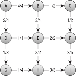
    Figure 14-12: Use a residual capacity network to find an augmenting path for this network.

11. ^**Expand the program you used in Exercise 9 to find the maximal flow between a source and sink node in a capacitated network.
12. Use the program you built for Exercise 11 to find an optimal work assignment for the network shown in Figure 14-9. What is the largest number of jobs that can be assigned?
13. To determine how robust a computer network is, you could calculate the number of different paths between two nodes. How could you use a maximal flow network to find the number of paths that don't share any links between two nodes? How could you find the number of paths that don't share links or nodes?
14. How many colors do you need to color a bipartite network? How many colors do you need to color a work assignment network?
15. ^**Expand the program you built for Exercise 12 to find the minimal flow cut between a source and sink node in a capacitated network.
16. Use the program you built for Exercise 15 to find a minimal flow cut for the network shown in Figure 14-12. What links are removed, and what is the cut's total capacity?