CHAPTER 4

Arrays

Arrays are extremely common data structures. They are intuitive, easy to use, and supported well by most programming languages. In fact, arrays are so common and well understood that you may wonder whether there's much to say about them in an algorithms book. Most applications use arrays in a relatively straightforward way, but special-purpose arrays can be useful in certain cases, so they deserve some attention here.

This chapter explains algorithmic techniques you can use to make arrays with nonzero lower bounds, save memory, and manipulate arrays more quickly than you can normally.

Basic Concepts

An array is a chunk of contiguous memory that a program can access by using indices—one index per dimension in the array. You can think of an array as an arrangement of boxes where a program can store values.

Figure 4-1 illustrates one-, two-, and three-dimensional arrays. A program can define higher-dimensional arrays, but trying to represent them graphically is hard.

Figure 4-1: You can think of one-, two-, and three-dimensional arrays as arrangements of boxes where a program can store values.

Typically a program declares a variable to be an array with a certain number of dimensions and certain bounds for each dimension. For example, the following code shows how a C# program might declare and allocate an array named numbers that has 10 rows and 20 columns:

In C#, array bounds are zero-based, so this array's row indices range from 0 to 9, and its column indices range from 0 to 19.

Behind the scenes the program allocates enough contiguous memory to hold the array's data. Logically the memory looks like a long series of bytes, and the program maps the array's indices to positions in this series of bytes, as explained in the following list:

• For one-dimensional arrays, the mapping from array indices to memory entries is simple: Index i maps to entry i.
• For two-dimensional arrays, the program can map the array entries in one of two ways: row-major order or column-major order:
  • In row-major order, the program maps the first row of array entries to the first set of memory locations. It then maps the second row to the set of memory locations after the first. It continues mapping one row at a time until all the entries are mapped.
  • In column-major order, the program maps the first column of array entries to the first set of memory locations. It then maps the second column to the second set of memory locations, and so forth.

Figure 4-2 shows row-major and column-major mappings.

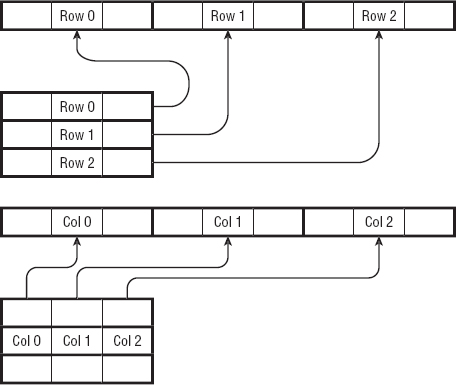
Figure 4-2: A program can map array entries to memory locations in either row-major or column-major order.

You can extend the ideas of row-major and column-major ordering for higher-dimensional arrays. For example, to store a three-dimensional array in row-major order, the program would map the first two-dimensional “slice” of the array where the third dimension's index is 0. It would map that slice in row-major order as usual. It would then similarly map the second slice where the third index is 1, and so on for the remaining slices.

Another way to think of this is as an algorithm for mapping a three-dimensional array. Suppose you have defined a Map2DArray method that maps a two-dimensional array. The following algorithm uses Map2DArray to map a three-dimensional array:

Similarly, you could use this algorithm to define algorithms for mapping arrays with even more dimensions.

Normally how a program maps array entries to memory locations is irrelevant to how a program works, and there's no reason why you should care. Your code manipulates the array entries, and you don't need to know how they are stored. However, understanding how the row-major and column-major orders work is useful when you try to create your own array-mapping data structures to implement triangular arrays. (Triangular arrays are discussed in the later section “Triangular Arrays.”)

One-dimensional Arrays

Algorithms that involve one-dimensional or linear arrays tend to be so straightforward that they're almost trivial. They often come up in programming interviews, however, so they're worth a brief discussion here. Linear array operations also provide a preview of operations used by more interesting data structures such as linked lists, stacks, and queues, so it's worth covering these operations now for completeness.

Finding Items

Chapter 7 covers some interesting algorithms for finding a target item in a sorted array. If the items in the array are not sorted, however, finding an item is a matter of performing a linear search or exhaustive search. You look at every element in the array until you find the target item or you conclude that the item is not in the array. The following algorithm finds a target item:

In the worst case, the target item may be the very last item in the array. So if the array has N items, the algorithm ends up examining all of them. That makes the algorithm's run time O(N).

The worst case also occurs if the target item is not in the array. In that case the algorithm must examine all N items to conclude that the item is not present.

If you were to successively search for every item in the array, the average search would take N/2 steps, which is still O(N).

Finding Minimum, Maximum, and Average

If the array contains numbers, you might want to find the minimum, maximum, and average values in the array. As is the case for finding an item, you cannot avoid looking at every item in the array when you want to find the minimum, maximum, or average.

The following algorithms find the minimum, maximum, and average values for a one-dimensional array of integers:

As is the case for the algorithm that finds a specific item, these algorithms must visit every item in the array, so they have run time O(N).

You can similarly calculate other statistical values such as the standard deviation and variance if you need them. One value that isn't as easy to calculate is the median, the value that lies in the middle of the values when they are sorted. For example, the median of 1, 3, 4, 7, 8, 8, 9 is 7 because there are three smaller values (1, 3, 4) and three larger values (8, 8, 9).

A single pass through the array won't give you all the information you need to calculate the median, because in some sense you need more global information about the values to find the median. You can't simply adjust a “running” median by looking at values one at a time.

One approach might be to think about each value in the list. For each test value, reconsider all the values, and keep track of those that are larger and smaller than the test value. If you find a test value where the number of smaller and larger entries is equal, the test value is the median.

The following is the basic algorithm:

This algorithm has a few flaws. For example, it doesn't handle the case in which multiple items have the same value, as in 1, 2, 3, 3, 4. It also doesn't handle arrays with an even number of items, which have no item in the middle. (If an array has an even number of items, its median is defined as the average of the two middlemost items. For example, the median of 1, 4, 6, 9 is 4 + 6 / 2 = 5.)

This algorithm isn't efficient enough to be worth fixing, but its run time is worth analyzing.

If the array contains N values, the outer For i loop executes N times. For every one of those iterations, the inner For j loop executes N times. That means the steps inside the inner loop execute N × N = N² times, giving the algorithm a run time of O(N²).

A much faster algorithm is to first sort the array and then find the median directly by looking at the values in the sorted array. Chapter 6 describes several algorithms for sorting an array containing N items in O(N log N) time. That's a lot faster than O(N²).

Inserting Items

Inserting an item at the end of a linear array is easy, assuming that the underlying programming language can extend the array by one item. Simply extend the array and insert the new item at the end.

Inserting an item anywhere else in the array is more difficult. The following algorithm inserts a new item at location position in a linear array:

Notice that this algorithm's For loop starts at the end of the array and moves toward the beginning. That lets it fill in the new position at the end of the array first and then fill each preceding spot right after its value has been copied to a new location.

If the array initially holds N items, this algorithm's For loop executes N − position times. In the worst case, when you're adding an item at the beginning of the array, position = 0 and the loop executes N times, so the algorithm's run time is O(N).

In practice, inserting items in a linear array isn't all that common, but the technique of moving over items in an array to make room for a new one is useful in other algorithms.

Removing Items

Removing the item with index k from an array is about as hard as adding an item. The code first moves the items that come after position k one position closer to the beginning of the array, and then the code resizes the array to remove the final unused entry.

In the worst case, when you're removing the first item from the array, the algorithm may need to move all the items in the array. That means it has a run time of O(N).

Nonzero Lower Bounds

Many programming languages require that all arrays use 0 for a lower bound in every dimension. For example, a linear array can have indices ranging from 0 to 9 but cannot have indices ranging from 1 to 10.

Sometimes, however, it's convenient to treat an array's dimension as if it had nonzero lower bounds. For example, suppose you're writing a sales program that needs to record sales figures for 10 employees with IDs between 1 and 10 for the years 2000 through 2010. In that case it might be nice to declare the array like this:

You can't do that in languages that require 0 lower bounds, but you can translate the more convenient bounds into bounds that start with 0 fairly easily. The following two sections explain how to use nonzero lower bounds for arrays with two or more dimensions.

Two Dimensions

Managing arrays with nonzero lower bounds isn't too hard for any given number of dimensions.

Consider again the example where you want an array indexed by employee ID and year, where employee ID ranges from 1 to 10 and year ranges from 2000 to 2010. These ranges include 10 employee ID values and 11 years, so they would allocate an array with 10 rows and 11 columns, as shown in the following pseudocode:

To access an entry for employee e in year y, you calculate the row and column in the actual array as follows:

Now the program simply works with the entry array[row, column].

This is easy enough, but you can make it even easier by wrapping the array in a class. You can make a constructor to give the object the bounds for its dimensions. It can then store the lower bounds so that it can later calculate rows and columns.

In some programming languages you can even make get and set methods to be the class's indexers, so you can treat objects almost as if they were arrays. For example, in C# you could use the following code to set and get values in an array:

The details of a particular programming language are specific to that language, so they aren't shown here. You can download the TwoDArray sample program from the book's website at www.wiley.com/go/essentialalgorithms to see the details in C#.

Higher Dimensions

The method described in the preceding section works well if you know the number of dimensions the array should have. Unfortunately, generalizing this technique for any number of dimensions is difficult because, for N dimensions, you need to allocate an N-dimensional array to hold the data. You could make separate classes to handle two, three, four, and more dimensions, but it would be better to find a more generalizable approach.

Instead of storing the values in a two-dimensional array, you could pack them into a one-dimensional array in row-major order. You would start by allocating an array big enough to hold all the items. If there are N rows and M columns, you would allocate an array with N × M entries:

To find an item's position in this array, first you calculate row and column as before. If an item corresponds to employee e and year y, the row and column are given by the following:

Now that you know the item's row and column, you need to find its index in the values array.

First, how many complete rows fit into the array before this item? If the item's row number is r, there are r complete rows before this item numbered 0, 1, ..., r − 1. Because there are <row size> items in each row, that means those rows account for r × <row size> items before this one.

Now, how many items come before this one in this item's row? If this item's column number is c, there are c items before this item in its row numbered 0, 1, ..., c − 1. Those items take up c positions in the values array.

The total number of items that come before this one in the values array is given by this:

Now you can find this item at values[index].

This technique is a bit more complicated than the technique described in the preceding section, but it is easier to generalize for any number of dimensions.

Suppose you want to create an array with N dimensions, with lower bounds stored in the lower_bounds array and with upper bounds stored in the upper_ bounds array.

The first step is to allocate a one-dimensional array with enough space to store all the values. Simply subtract each lower bound from each upper bound to see how “wide” the array must be in that dimension, and then multiply the resulting “widths” together:

The next step, mapping row and column to a position in the one-dimensional array, is a bit more confusing. Recall how the preceding example mapped row and column to an index in the values array. First the code determined how many complete rows belonged in the array and multiplied that number by the number of items in a row. The code then added 1 for each position in the item's row that was before the item.

Moving to three dimensions isn't much harder. Figure 4-3 shows a 4×4×3 three-dimensional array with dimensions labeled height, row, and column. The entry with coordinates (1, 1, 3) is highlighted in gray.

Figure 4-3: The first step in mapping an item to the values array is determining how many complete “slices” come before it.

To map the item's coordinates (1, 1, 3) to an index in the values array, first determine how many complete “slices” come before the item. Because the item's height coordinate is 1, there is one complete slice before the item in the array. The size of a slice is <row size> × <column size>. If the item has coordinates (h, r, c), the number of items that come before this one due to slices is given by the following:

Next you need to determine how many items come before this one due to complete rows. In this example, the item's row is 1, so one row comes before the item in the values array. If the item has row r, you need to add r times the size of a row to the index:

Finally, you need to add 1 for each item that comes before this one in its column. If the item has column c, this is simply c:

You can extend this technique to work in even higher dimensions. To make calculating indices in the values array easier, you can make a slice_sizes array that holds the size of the “slice” at each of the dimensions. In the three-dimensional case, these values are <row size> × <column size>, <column size>, and 1.

To move to higher dimensions, you can find a slice size by multiplying the next slice size by the size of the current dimension. For example, for a four-dimensional array, the next slice size would be <height size> × <row size> × <column size>.

With all this background, you're ready to see the complete algorithm. Suppose the bounds array holds alternating lower and upper bounds for the desired N-dimensional array. Then the following pseudocode initializes the array:

This code calculates the number of dimensions by dividing the number of values in the bounds array by 2. It creates a LowerBound array to hold the lower bounds and a SliceSize array to hold the sizes of slices at different dimensions.

Next the code sets slice_size to 1. This is the size of the slice at the highest dimension, which is a column in the preceding example.

The code then loops through the dimensions, starting at the highest and looping toward dimension 0. (This corresponds to looping from column to row to height in the preceding example.) It sets the current slice size to slice_size and saves the dimension's lower bound. It then multiplies slice_size by the size of the current dimension to get the slice size for the next-smaller dimension.

After it finishes looping over all the dimensions, slice_size holds the sizes of all the array's dimensions multiplied together. That is the total number of items in the array, so the code uses it to allocate the Values array, where it will store the array's values.

The following deceptively simple pseudocode uses the LowerBound and SliceSize arrays to map the indices in the indices array to an index in the Values array:

The code initializes index to 0. It then loops over the array's dimensions. For each dimension, it multiplies the number of slices at that dimension by the size of a slice at that dimension and adds the result to index.

After it has looped over all the dimensions, index holds the item's index in the Values array.

You can make using the algorithm easier by encapsulating it in a class. The constructor can tell the object what dimensions to use. Depending on your programming language, you may be able to make get and set methods that are used as accessors so that a program can treat an object as if it actually were an array.

Download the NDArray sample program from the book's website to see a C# implementation of this algorithm.

Triangular Arrays

Some applications can save space by using triangular arrays instead of normal rectangular arrays. In a triangular array, the values above the diagonal (where the item's column is greater than its row) have some default value, such as 0, null, or blank. Figure 4-4 shows an upper triangular array.

For example, a connectivity matrix represents the connections between points in some sort of network. The network might be an airline's flight network that indicates which airports are connected to other airports. The array's entry connected[i, j] is set to 1 if there is a flight from airport i to airport j. If you assume that there is a flight from airport j to airport i whenever there is a flight from airport i to airport j, connected[i, j] = connected[j, i]. In that case there's no need to store both connected[i, j] and connected[j, i] because they are the same.

Figure 4-4: In a triangular array, values above the diagonal have a default value.

In cases such as this, the program can save space by storing the connectivity matrix in a triangular array.

Building a triangular array isn't too hard. Simply pack the array's values into a one-dimensional array, skipping the entries that should not be included. The challenges are to figure out how big the one-dimensional array must be and to figure out how to map rows and columns to indices in the one-dimensional array.

Table 4-1 shows the number of entries needed for triangular arrays of different sizes.

Table 4-1: Entries in Triangular Arrays

NUMBER OF ROWS	NUMBER OF ENTRIES
1	1
2	3
3	6
4	10
5	15
6	21
7	28

If you study Table 4-1, you'll see a pattern. The number of cells needed for N rows equals the number needed for N − 1 rows plus N.

If you think about triangular arrays for a while, you'll realize that they contain roughly half the number of the entries in a square array with the same number of rows. A square array containing N rows holds N² entries, so it seems likely that the number of entries in the corresponding triangular array would involve N². If you start with a general quadratic equation A × N² + B × N + C and plug in the values from Table 4-1, you can solve for A, B, and C to find that the equation is (N² + N) / 2.

That solves the first challenge. To build a triangular array with N rows, allocate a one-dimensional array containing (N² + N) / 2 items.

The second challenge is to figure out how to map rows and columns to indices in the one-dimensional array. To find the index for an entry with row r and column c, you need to figure out how many entries come before that one in the one-dimensional array.

To answer that question, look at the array shown in Figure 4-5 and consider the number of entries that come before entry (3, 2).

Figure 4-5: To find the index of an entry, you must figure out how many entries come before it in the one-dimensional array.

The entries due to complete rows are highlighted with a thick border in Figure 4-5. The number of those entries is the same as the number of all entries in a triangular array with three rows, and you already know how to calculate that number.

The entries that come before the target entry (3, 2) that are not due to complete rows are those to the left of the entry in its row. In this example, the target entry is in column 2, so there are two entries to its left in its row.

In general, the formula for the index of the entry with row r and column c is ((r − 1)² + (r − 1)) / 2 + c.

With these two formulas, working with triangular arrays is easy. Use the first formula, (N² + N) / 2, to figure out how many items to allocate for an array with N rows. Use the second formula, ((r − 1)² + (r − 1)) / 2 + c, to map rows and columns to indices in the one-dimensional array, as shown in the following pseudocode:

You can make this easier by wrapping the triangular array in a class. If you can make the get and set methods indexers for the class, a program can treat a triangular array object as if it were a normal array.

One last detail is how the triangular array class should handle requests for entries that do not exist in the array. For example, what should the class do if the program tries to access entry (1, 4), which lies in the missing upper half of the array? Depending on the application, you might want to return a default value, switch the row and column and return that value, or throw an exception.

Sparse Arrays

Triangular arrays let a program save memory if you know that the array will not need to hold values above its diagonal. If you know an array will hold very few entries, you may be able to save even more memory.

For example, consider again an airline connectivity matrix that holds a 1 in the [i, j] entry to indicate that there is a flight between city i and city j. The airline might have only 600 flights connecting 200 cities. In that case there would be only 600 nonzero values in an array of 40,000 entries. Even if the flights are symmetrical (for every i−j flight there is a j−i flight) and you store the connections in a triangular array, the array would hold only 300 nonzero entries out of a total of 20,100 entries. The array would be almost 99% unused.

A sparse array lets you save even more space by not representing the missing entries. To get an item's value, the program searches for the item in the array. If the item is present, the program returns its value. If the item is missing, the program returns a default value for the array. (For the connectivity matrix example, the default value would be 0.)

One way to implement a sparse array is to make a linked list of linked lists. The first list holds information about rows. Each item in that list points to another linked list holding information about entries in the array's columns for that row.

You can build a sparse array with two cell classes—an ArrayRow class to represent a row and an ArrayEntry class to represent a value in a row.

The ArrayRow class stores a row number, a reference or pointer to the next ArrayRow, and a reference to the first ArrayEntry in that row. The following shows the ArrayRow class's layout:

The ArrayEntry class stores the entry's column number, whatever value the entry should hold for the array, and a reference to the next ArrayEntry object in this row. The following shows the ArrayEntry class's layout, where T is whatever type of data the array must hold:

To make adding and removing rows easier, the list of rows can start with a sentinel, and each list of values in a row can start with a sentinel. Figure 4-6 shows a sparse array with the sentinels shaded.

To make it easier to determine when a value is missing from the array, the ArrayRow objects are stored in increasing order of RowNumber. If you're searching the list for a particular row number and you find an ArrayRow object that has a lower RowNumber, you know that the row number you're looking for isn't in the array.

Similarly, the ArrayEntry objects are stored in increasing order of ColumnNumber.

Note that the RowEntry objects that seem to be aligned vertically in Figure 4-6 do not necessarily represent the same columns. The first RowEntry object in the first row might represent column 100, and the first RowEntry object in the second row might represent column −50.

The arrangement shown in Figure 4-6 looks complicated, but it's not too hard to use. To find a particular value, look down the row list until you find the right row. Then look across that row's value list until you find the column you want. If you fail to find the row or column, the value isn't in the array.

This arrangement requires some ArrayRow objects and sentinels that don't hold values, but it's still more efficient than a triangular array if the array really is sparse. For example, in the worst case a sparse array would contain one value in each row. In that case an N × N array would use N + 1 ArrayRow objects and 2 × N ArrayEntry objects. Of those objects, only N would contain actual values, and the rest would be sentinels or used to navigate through the array. The fraction of objects containing array values is N / (N + 1 + 2 * N) = N / (3 * N + 1), or approximately 1/3. Compare that to the triangular array described previously, which was almost 99% empty.

Figure 4-6: Adding and removing cells is easier if each linked list begins with a sentinel.

With the data structure shown in Figure 4-6, you still need to write algorithms to perform three array operations:

1. Get the value at a given row and column or return a default value if the value isn't present.
2. Set a value at a given row and column.
3. Delete the value at a given row and column.

These algorithms are a bit easier to define if you first define methods for finding a particular row and column.

Find a Row or Column

To make finding values easier, you can define the following FindRowBefore method. This method finds the ArrayRow object before the spot where a target row should be. If the target row is not in the array, this method returns the ArrayRow before where the target row would be if it were present:

This algorithm sets variable array_row equal to the array's row sentinel. The algorithm then repeatedly advances array_row to the next ArrayRow object in the list until either the next object is null or the next object's RowNumber is at least as large as the target row number.

If the next object is null, the program has reached the end of the row list without finding the desired row. If the row were present, it would belong after the current array_row object.

If the next object's RowNumber value equals the target row, the algorithm has found the target row.

If the next object's RowNumber value is greater than the target row, the target row is not present in the array. If the row were present, it would belong after the current array_row object.

Similarly, you can define a FindColumnBefore method to find the ArrayEntry object before the spot where a target column should be. This method takes as parameters the target column number and the sentinel for the row that should be searched for that number:

If the array holds N ArrayRow objects, the FindRowBefore method takes O(N) time. If the row holding the most nondefault items contains M of those items, the FindColumnBefore method runs in O(M) time. The exact run time for these methods depends on the number and distribution of nondefault values in the array.

Get a Value

Getting a value from the array is relatively easy once you have the FindRowBefore and FindColumnBefore methods:

This algorithm uses FindRowBefore to set array_row to the row before the target row. It then advances array_row to the next row, hopefully the target row. If array_row is null or refers to the wrong row, the GetValue method returns the array's default value.

If the algorithm finds the correct row, it uses FindColumnBefore to set array_ entry to the column before the target column. It then advances array_entry to the next column, hopefully the target column. If array_entry is null or refers to the wrong column, the GetValue method returns the array's default value.

If the algorithm gets this far, it has found the correct ArrayEntry object, so it returns that object's value.

This algorithm calls the FindRowBefore and FindColumnBefore methods. If the array has N rows that contain nondefault values, and the row with the most nondefault values contains M of those values, the total run time for the GetValue method is O(N + M). This is much longer than the O(1) time needed to get a value from a normal array, but the sparse array uses much less space.

Set a Value

Setting a value is similar to finding a value, except that the algorithm must be able to insert a new row or column into the array if necessary:

The algorithm starts by checking the value it is setting in the array. If the value is the default value, the program should delete it from the array to minimize the array's size. To do that, it calls the DeleteEntry method, described in the next section, and returns.

If the new value isn't the default value, the algorithm calls the FindRowBefore method to find the row before the target row. If the row after the one returned by FindRowBefore isn't the target row, either the algorithm reached the end of the row list, or the next row comes after the target row. In either case the algorithm inserts a new ArrayRow object between the row before and the row that follows it.

Figure 4-7 shows this process. In the list on the left, the target row is missing but should go where the dashed ellipse is.

Figure 4-7: If the target row is missing, the SetValue method inserts a new ArrayRow.

To insert the new ArrayRow object, the algorithm creates the new object and sets its NextRow reference to the array_row object's NextRow value. It then gives the new object a new row sentinel.

When it has finished, the list looks like the right side of Figure 4-7, with array_row's NextRow reference pointing to the new object.

Having found the target row, creating it if necessary, the algorithm calls the FindColumnBefore method to find the ArrayEntry object that represents the target column. If that object doesn't exist, the algorithm creates it and inserts it into the linked list of the ArrayEntry object, much as it inserted the ArrayRow if necessary.

Finally, the algorithm moves the variable array_entry to the ArrayEntry corresponding to the row and sets its value.

The SetValue algorithm may call the DeleteEntry algorithm, described in the following section. That algorithm calls the FindRowBefore and FindColumnBefore methods. If the SetValue algorithm does not call DeleteEntry, it calls FindRowBefore and FindColumnBefore. In either case, the method calls FindRowBefore and FindColumnBefore either directly or indirectly.

Suppose the array has N rows that contain nondefault values and the row with the most nondefault values contains M of those values. In that case, those FindRowBefore and FindColumnBefore methods give the SetValue algorithm a total run time of O(N + M).

Delete a Value

The algorithm to delete a value follows the same general approach used to get or set a value:

This algorithm calls FindRowBefore to find the row before the target row. If the target row doesn't exist, the algorithm doesn't need to delete anything, so it returns.

Next the algorithm calls FindColumnBefore to find the column before the target column in the target row. If the target column doesn't exist, again the algorithm doesn't need to delete anything, so it returns.

At this point, the algorithm has found the ArrayEntry object before the target entry in the row's linked list of entries. It removes the target entry from the list by setting the NextColumn reference of the previous entry to refer to the object after the target entry.

This operation is shown in Figure 4-8. The list at the top is the original list. The variable array_entry refers to the entry before the target entry. To remove the target entry, the algorithm makes that entry's NextColumn reference point to the following entry.

Figure 4-8: To remove a target entry, the algorithm sets the preceding entry's NextColumn reference to the entry after the target entry.

The algorithm does not change the target entry's NextColumn reference. That reference still refers to the following entry, but the algorithm no longer has a reference that can refer to the target entry, so it is essentially lost to the program.

After it has removed the target entry from the row's linked list, the program examines the row's ArrayRow sentinel. If that object's NextColumn reference is not null, the row still holds other column entries, so the algorithm is finished, and it returns.

If the target row no longer contains any entries, the algorithm removes it from the linked list of ArrayRow objects, much as it removed the target column entry.

The DeleteEntry algorithm calls FindRowBefore and FindColumnBefore. If the array has N rows that contain nondefault values and the row with the most nondefault values contains M of those values, the total run time for the DeleteEntry method is O(N + M).

Matrices

One application of arrays is to represent matrices. If you use normal arrays, it's fairly easy to perform operations on matrices. For example, to add two 3×3 matrices you simply add the corresponding entries. The algorithm following the next note shows this operation for two normal two-dimensional arrays.

The following algorithm shows how you can multiply two normal two-dimensional matrices:

These algorithms work with triangular or sparse arrays, but they are inefficient because they examine every item in both input arrays even if those entries aren't present.

For example, a triangular array is missing all values [i, j] where j > i, so adding or multiplying those entries takes on special meaning. If the missing entries are assumed to be 0, adding or multiplying them doesn't add to the result. (If those entries are assumed to have some other default value, adding or multiplying the arrays will result in a nontriangular array, so you may need to add or multiply the arrays out completely.)

Instead of considering every entry, the algorithms should consider only the entries that are actually present. For triangular arrays, this isn't too confusing. Writing addition and multiplication algorithms for triangular arrays are topics saved for Exercises 12 and 13. If you get stuck on them, you can read the solutions in Appendix B.

The situation is a bit more confusing for sparse arrays, but the potential time savings is even greater. For example, when you add two sparse matrices, there's no need to iterate over rows and columns that are not present in either of the input arrays.

The following high-level algorithm adds two sparse matrices:

Similarly, you can write an algorithm to multiply two sparse matrices without examining all the missing rows and columns. This is saved for Exercise 15. If you get stuck writing that algorithm, read the solution in Appendix B.

Summary

Normal arrays are simple, intuitive, and easy to use, but for some applications they can be awkward. In some applications it may be more natural to work with an array that has nonzero lower bounds. By using the techniques described in the section “Nonzero Lower Bounds,” you can effectively do just that.

Normal arrays are also inefficient for some applications. If an array holds entries in only its lower-left half, you can use a triangular array to save roughly half of the array's memory. If an array contains even fewer entries, you may be able to save even more space by using a sparse array.

Arrays with nonzero lower bounds, triangular arrays, and sparse arrays are more complicated than the normal arrays provided by most programming languages, but in some cases they offer greater convenience and large memory savings.

An array provides random access to the elements it contains. It lets you get or set any item if you know its indices in the array.

The next chapter explains two different kinds of containers: stacks and queues. Like arrays, these data structures hold collections of items. Unlike arrays, with their random access behavior, however, they have very constrained methods for inserting and removing items.

Exercises

Asterisks indicate particularly difficult problems.

1. Write an algorithm to calculate the sample variance of a one-dimensional array of numbers where the sample variance for an array containing N items is defined by this equation:

   

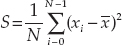
   Hare is the mean (average) of the values in the array, and the summation symbol Σ means to add up all the x_i values as i varies from 0 to N − 1.

2. Write an algorithm to calculate the sample standard deviation of a one-dimensional array of numbers where the sample standard deviation is defined to be the square root of the sample variance.
3. Write an algorithm to find the median of a sorted one-dimensional array. (Be sure to handle arrays holding an even or odd number of items.)
4. The section “Removing Items” explained how to remove an item from a linear array. Write the algorithm in pseudocode.
5. The triangular arrays discussed in this chapter are sometimes called “lower triangular arrays” because the values are stored in the lower-left half of the array. How would you modify that kind of array to produce an upper triangular array with the values stored in the upper-right corner?
6. How would you modify the lower triangular arrays described in this chapter to make an “upper-left” array where the entries are stored in the upper-left half of the array? What is the relationship between row and column for the entries in the array?
7. Suppose you define the main diagonal of a rectangular (and nonsquare) array to start in the upper-left corner and extend down and to the right until it reaches the bottom or right edge of the array. Write an algorithm that fills entries on or below the main diagonal with 1s and entries above the main diagonal with 0s.
8. Consider the diagonal of a rectangular array that starts in the last column of the first row and extends left and down until it reaches the bottom or left edge of the array. Write an algorithm that fills the entries on or above the diagonal with 1s and entries below the diagonal with 0s.
9. Write an algorithm that fills each item in a rectangular array with the distance from that entry to the nearest edge of the array.
10. ^*Generalize the method for building triangular arrays to build three-dimensional tetrahedral arrays that contain entries value[i, j, k] where j ≤ i and k ≤ j. How would you continue to extend this method for even higher dimensions?
11. How could you make a sparse triangular array?
12. Write an algorithm that adds two triangular arrays.
13. Write an algorithm that multiplies two triangular arrays.
14. The algorithm described for adding two sparse matrices is fairly high-level. Expand the algorithm to provide details in place of the instructions inside the angle brackets (<>). (Hint: You may want to make a separate CopyEntries method to copy entries from one list to another and a separate AddEntries method to combine the entries in two rows with the same row number.)
15. At a high level, write an algorithm that efficiently multiplies two sparse matrices that have default value 0.