CHAPTER 13

Basic Network Algorithms

Chapters 10 through 12 explained trees. This chapter describes a related data structure: the network. Like a tree, a network contains nodes that are connected by links. Unlike the nodes in a tree, the nodes in a network don't necessarily have a hierarchical relationship. In particular, the links in a network may create cycles, so a path that follows the links could loop back to its starting position.

This chapter explains networks and some basic network algorithms, such as detecting cycles, finding shortest paths, and finding a tree that is part of the network that includes every node.

Network Terminology

Network terminology isn't quite as complicated as tree terminology, because it doesn't borrow as many terms from genealogy, but it's still worth taking a few minutes to review the relevant terms.

A network consists of a set of nodes connected by links. (Sometimes, particularly when you're working on mathematical algorithms and theorems, a network is called a graph, nodes are called vertices, and links are called edges.) If node A and node B are directly connected by a link, they are adjacent and are called neighbors.

Unlike the case with a tree, a network has no root node, although there may be particular nodes of interest, depending on the network. For example, a transportation network might contain special hub nodes where buses, trains, ferries, or other vehicles start and end their routes.

A link can be undirected (you can traverse it in either direction) or directed (you can traverse it in one direction only). A network is called a directed or undirected network depending on what kinds of links it contains.

A path is an alternating sequence of nodes and links through the network from one node to another. Suppose there is only one link from any node to any adjacent node (in other words, there aren't two links from node A to node B). In that case, you can specify a path by listing either the nodes it visits or the links it uses.

A cycle or loop is a path that returns to its starting point.

As is the case with trees, the number of links that leave a node is called the node's degree. The degree of the network is the largest degree of any of the nodes in it. In a directed network, a node's in-degree and out-degree are the numbers of links entering and leaving the node.

Nodes and links often have data associated with them. For example, nodes often have names, ID numbers, or physical locations such as a latitude and longitude. Links often have associated costs or weights, such as the time it takes to drive across a link in a street network. They may also have maximum capacities, such as the maximum amount of current you can send over a wire in a circuit network or the maximum number of cars that can cross a link in a street network per unit of time.

A reachable node is a node that you can reach from a given node by following links. Depending on the network, you may be unable to reach every node from every other node.

In a directed network, if node B is reachable from node A, nodes A and B are said to be connected. Note that if node A is connected to node B, and node B is connected to node C, node A must be connected to node C.

A connected component of a network is a set of all the nodes that are mutually connected. The network is called connected if all its nodes are connected to each other.

If a directed network's nodes are all connected, the network is called strongly connected. If a directed network is connected if you replace its directed links with undirected links, the network is weakly connected.

Figure 13-1 shows some of the parts of a small directed network. Arrows represent the links, and the arrowheads indicate the links' directions. Double-headed arrows represent pairs of links that go in opposite directions.

The numbers on the links are the links' costs. This example assumes that opposite links have the same costs. That need not be the case, but then drawing the network is harder.

The network shown in Figure 13-1 is strongly connected because you can find a path using links from any node to any other node.

Figure 13-1: In a directed network, arrows show the directions of links.

Notice that paths between nodes may not be unique. For example, A-E-F and A-B-C-F are both paths from node A to node F.

Table 13-1 summarizes these tree terms to make remembering them a bit easier.

Table 13-1 Summary of Network Terminology

TERM	MEANING
adjacent	If two nodes are connected by a link, they are adjacent.
capacity	The maximum amount of something that can move through a node or link, such as the maximum current that can flow through a wire in an electrical network or the maximum number of cars that can move through a link in a street network per unit of time.
connected	In an undirected network, nodes A and B are connected if node B is reachable from node A and vice versa. An undirected network is connected if every node is reachable from every other node.
connected component	A set of nodes that are mutually connected.
cost	A link may have an associated cost. Less commonly, a node may have a cost.
cycle	A path that returns to its starting point.
degree	In an undirected network, the number of links leaving a node. In a directed network, a node has an in-degree and an out-degree.
directed	A link is directed if you can traverse it in only one direction. A network is directed if it contains directed links.
edge	Link.
graph	Network.
in-degree	In a directed network, the number of links entering a node.
link	An object in a network that represents a relationship between two nodes. Links can be directed or undirected.
loop	Cycle.
neighbor	Two nodes are neighbors if they are adjacent.
node	An object in a network that represents a point-like location. Nodes are connected by links.
out-degree	In a directed network, the number of links leaving a node.
path	An alternating series of nodes and links that leads from one node to another. If there is only one link from any node to an adjacent node, you can specify a path by listing the nodes or links it includes.
reachable node	Node B is reachable from node A if there is a path from node A to node B.
strongly connected	A directed network is strongly connected if every node is reachable from every other node.
undirected	A link is undirected if you can traverse it only in either direction. A network is undirected if it contains only undirected links.
vertex	Node.
weakly connected	A directed network is weakly connected if every node is reachable from every other node when you replace the directed links with undirected links.
weight	Cost.

Network Representations

It's fairly easy to use objects to represent a network. You can represent nodes with a node class.

How you represent links depends on how you will use them. For example, if you are building a directed network, you can make the links be references stored inside the node class. If the links should have costs or other data, you can also add that to the node class. The following pseudocode shows a simple node class for this situation:

This representation works for simple problems, but often it's useful to make a class to represent the links like objects. For example, some algorithms, such as the minimal spanning tree algorithm described later in this chapter, build lists of links. If the links are objects, it's easy to place specific links in a list. If the links are represented by references stored in the node class, it's harder to put them in lists.

The following pseudocode shows node and link classes that store links as separate objects for an undirected network:

Here the Link class contains an array of two Node objects representing the nodes it connects.

In an undirected network, a Link object represents a link between two nodes, and the ordering of the nodes doesn't matter. If a link connects node A and node B, the Link object appears in the Neighbors list for both nodes, so you can follow it in either direction.

Because the order of the nodes in the link's Nodes array doesn't matter, an algorithm trying to find a neighbor must compare the current node to the link's Nodes to see which one is the neighbor. For example, if an algorithm is trying to find the neighbors of node A, it must look at a link's Nodes array to see which entry is node A and which entry is the neighbor.

In a directed network, the link class only really needs to know its destination node. The following pseudocode shows classes for this situation:

However, it may still be handy to make the link class contain references to both of its nodes. For example, if the network's nodes have spatial locations, and the links have references to their source and destination nodes, it is easier for the links to draw themselves. If the links store only references to their destination nodes, the node objects must pass extra information to a link to let it draw itself.

If you use a link class that uses the Nodes array, you can store the node's source node in the array's first entry and its destination node in the array's second entry.

The best way to represent a network in a file depends on the tools available in your programming environment. For example, even though XML is a hierarchical language and works most naturally with hierarchical data structures, some XML libraries can save and load network data.

To keep things simple, the examples that are available for download use a simple text file structure. The file begins with the number of nodes in the network. After that, the file contains one line of text per node.

Each node's line contains the node's name and its x- and y-coordinates. Following that is a series of entries for the node's links. Each link's entry includes the index of the destination node, the link's cost, and the link's capacity.

The following lines show the format:

For example, the following is a file representing the network shown in Figure 13-2:

The file begins with the number of nodes, 3. It then contains lines representing each node.

The line for node A begins with its name, A. The next two entries give the node's x- and y-coordinates, so this node is at location (85, 41).

The line then contains a sequence of sets of values describing links. The first set of values means the first link leads to node B (index 1), has a cost of 87, and has a capacity of 1. The second set of values means the second link leads to node C (index 2), has a cost of 110, and has a capacity of 4.

The file's other lines define nodes B and C and their links.

Figure 13-2: This network contains four links—two connecting node A to nodes B and C, and two connecting node B to node C.

Traversals

Many algorithms traverse a network in some way. For example, the spanning tree and shortest-path algorithms all visit the nodes in a tree.

The following sections describe several algorithms that use different kinds of traversals to solve network problems.

Depth-first Traversal

The preorder traversal algorithm for trees described in Chapter 10 almost works for networks. The following pseudocode shows that algorithm modified slightly to use a network node class:

The method first processes the current node. It then loops through the node's links and recursively calls itself to process each link's destination node.

This would work except for one serious problem. Unlike trees, networks are not hierarchical, so they may contain cycles. If a network contains a cycle, this algorithm will end up in an infinite loop, recursively following the cycle.

One solution to this problem is to give the algorithm a way to tell if it has visited a node before. An easy way to do that is to add a Visited property to the node class. The following pseudocode shows the algorithm rewritten to use a Visited property:

Now the algorithm visits the current node and sets its Visited property to True. It then loops through the node's links. If the Visited property of the link's destination node is False, it recursively calls itself to process that destination node.

This version works but may lead to very deep levels of recursion. If a network contains N nodes, the algorithm might call itself N times. If N is large, that could exhaust the program's stack space and make the program crash.

You can avoid this problem if you use the techniques described in Chapter 9 to remove the recursion. The following pseudocode shows a version that uses a stack instead of recursion:

This algorithm visits the start node and pushes it onto a stack. Then, as long as the stack isn't empty, it pops the next node off the stack and processes it.

To process a node, the algorithm examines the node's links. If a link's destination node has not been visited, the algorithm marks it as visited and adds it to the stack for later processing.

Because of how this algorithm pushes nodes onto a stack, it traverses the network in a depth-first order. To see why, suppose the algorithm starts at node A and that A has neighbors B₁, B₂, and so on. When the algorithm processes node A, it pushes the neighbors onto the stack. Later, when it processes neighbor B₁, it pushes that node's neighbors C₁, C₂, and so on onto the stack. Because the stack returns items in last-in-first-out order, the algorithm processes the C_i nodes before it processes the B_i nodes. As it continues, the algorithm moves quickly through the network, traveling long distances away from the start node A before it gets back to processing that node's closer neighbors.

Because the traversal visits nodes far from the root node before it visits all the ones that are closer to the root, this is called a depth-first traversal.

Figure 13-3 shows a depth-first traversal with the nodes labeled according to the order in which they were traversed.

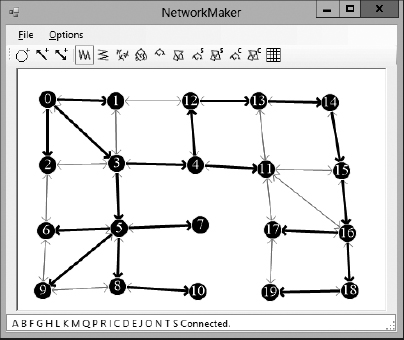
Figure 13-3: In a depth-first traversal, some nodes far from the start node are visited before some nodes close to the start node.

With some work, you can figure out how the nodes were added to the traversal. The algorithm started with the node labeled 0. It then added the nodes labeled 1, 2, and 3 to its stack.

Because node 3 was added to the stack last, it was processed next, and the algorithm added nodes 4 and 5 to the stack. Because node 5 was added last, the algorithm processed it next and added nodes 6, 7, 8, and 9 to the stack.

If you like, you can continue studying Figure 13-3 to figure out why the algorithm visited the nodes in the order it did. But at this point you should be able to see how some nodes far from the start node are processed before some of the nodes closer to the start node.

Breadth-first Traversal

In some algorithms, it is convenient to traverse nodes closer to the start node before the nodes that are farther away. The previous algorithm visited some nodes far from the start node before it visited some closer nodes because it used a stack to process the nodes. If you use a queue instead of a stack, the nodes are processed in first-in-first-out order, and the nodes closer to the start node are processed first.

Because this algorithm visits all of a node's neighbors before it visits any other nodes, this is called a breadth-first search. Figure 13-4 shows a breadth-first traversal with the nodes labeled according to the order in which they were traversed.

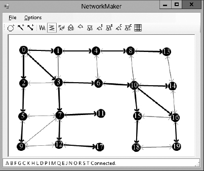
Figure 13-4: In a breadth-first traversal, nodes close to the starting node are visited before those that are farther away.

As with the depth-first traversal, you can study Figure 13-4 to see how the algorithm visited the network's nodes. The algorithm started with the node labeled 0. It then added its neighbors labeled 1, 2, and 3 to its queue.

Because the queue returns items in first-in-first-out order, the algorithm next processes node 1 and adds its neighbors to the queue. The only neighbor of that node that has not been visited yet is node 4.

Next the algorithm removes node 2 from the queue and adds its neighbor, marked 5, to the queue. It then removes the node marked 3 from the queue and adds its neighbors 6 and 7 to the queue.

If you like, you can continue studying Figure 13-4 to figure out why the algorithm visited the nodes in the order it did. But at this point you should be able to see that all the nodes closest to the start node were visited before any of the nodes farther away.

Connectivity Testing

The traversal algorithms described in the previous two sections immediately lead to a couple other algorithms with only minor modifications. For example, a traversal algorithm visits all the nodes that are reachable from the start node. For an undirected network, that means it visits every node in the network if the network is connected. This leads to the following simple algorithm to determine whether an undirected network is connected:

This algorithm uses the previous traversal algorithm and then checks each node's Visited property to see if it was visited.

You can extend this algorithm to find all the network's connected components. Simply use the traversal algorithm repeatedly until you visit all the nodes. The following pseudocode shows an algorithm that uses a depth-first traversal to find the network's connected components.:

This algorithm returns a list of lists, each holding the nodes in a connected component. It starts by making the variable num_visited to keep track of how many nodes have been visited. It then makes the list of lists it will return.

The algorithm then enters a loop that continues as long as it has not visited every node. Inside the loop the program finds a node that has not yet been visited, adds it to a stack as in the traversal algorithm, and also adds it to a new list of nodes that represents the node's connected component.

The algorithm then enters a loop similar to the one the earlier traversal algorithm used to process the stack until it is empty. The only real difference is that this algorithm adds the nodes it visits to the list it is currently building in addition to adding them to the stack.

When the stack is empty, the algorithm has visited all the nodes that are connected to the start node. At that point it finds another node that hasn't been visited and starts again.

When every node has been visited, the algorithm returns the list of connected components.

Spanning Trees

If an undirected network is connected, you can make a tree rooted at any node, showing a path from the root node to every other node in the network. This tree is called a spanning tree because it spans all the nodes in the network.

For example, Figure 13-5 shows a spanning tree rooted at node H for a network. If you follow the darker links, you can trace a path from the root node H to any other node in the network. For example, the path to node M visits nodes H, C, B, A, F, K, L, and M.

Figure 13-5: A spanning tree connects all the nodes in a network.

The traversal algorithms described earlier actually find spanning trees but they just don't record which links were used in the tree. To modify the previous algorithms to record the links used, simply add the following lines right after the statement that marks a new node as visited:

Basically the algorithm starts with the root node in the spanning tree. At each step, it picks another node that is adjacent to the spanning tree and adds it to the tree. The new algorithm simply records which links were used to connect the nodes to the growing spanning tree.

Minimal Spanning Trees

The spanning tree algorithm described in the preceding section lets you use any node in the network as the root of a spanning tree, so many spanning trees are possible.

A spanning tree that has the least possible cost is called a minimal spanning tree. Note that a network may have more than one possible minimal spanning tree. In fact, if all the links in the network have the same cost, every spanning tree is a minimal spanning tree.

The following steps describe a simple high-level algorithm for finding a minimal spanning tree with root node R:

1. Add the root node R to the initial spanning tree.
2. Repeat until every node is in the spanning tree:
   1. Find a least-cost link that connects a node in the spanning tree to a node that is not yet in the spanning tree.
   2. Add that link's destination node to the spanning tree.

The algorithm is greedy because at each step it selects a link that has the least possible cost. By making the best choices locally, it achieves the best solution globally.

For example, consider the network shown on the left in Figure 13-6, and suppose the bold links and nodes are part of a growing spanning tree rooted at node A. In step 2a, you examine the links that connect nodes in the tree with nodes that are not yet in the tree. In this example, those links have costs 15, 10, 12, and 11. Using the greedy algorithm, you add the least-cost link, which has cost 10, to get the tree on the right.

The most time-consuming step in this algorithm is step 2a, finding the next link to add to the tree. How much time this step takes depends on the approach you use.

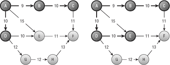
Figure 13-6: At each step, you add to the spanning tree the least-cost link that connects a node in the tree to a node that is not in the tree.

One way to find a least-cost link is to loop through the tree's nodes, examining their links to find one that connects to a node outside the tree and that has minimal cost. This is fairly time-consuming, because the algorithm must examine the links of the tree's nodes many times, even if they lead to other nodes that are already in the tree.

A better approach is to keep a list of candidate links. When the algorithm adds a node to the growing spanning tree, it also adds any links from that node to a node outside the tree to the candidate list. To find a minimal link, the algorithm looks through the list for the smallest link. As it searches the list, if it finds a link that leads to another node that is already in the tree (because that node was added to the tree after the link was added to the candidate list), the algorithm removes it from the list. That way, the algorithm doesn't need to consider the link again later. When the candidate list is empty, the algorithm is done.

Finding Paths

Finding paths in a network is a common task. An everyday example is finding a route from one location to another in a street network.

The following sections describe some algorithms for finding paths through networks.

Finding Any Path

The spanning tree algorithms described earlier in this chapter give you a method for finding a path between any two nodes in a network. The following steps describe a simple high-level algorithm for finding a path from node A to node B in a network:

1. Find a spanning tree rooted at node A.
2. Follow the reversed links in the spanning tree from node B to node A.
3. Reverse the order in which the links were followed.

The algorithm builds the spanning tree rooted at node A. Then it starts at node B. For each node in its path, it finds the link in the spanning tree that leads to that node. It records that link and moves to the next node in the path.

Unfortunately, finding the link that leads to a particular node in the spanning tree is difficult. Using the spanning tree algorithms described so far, you would need to loop through every link to determine whether it was part of the spanning tree and whether it ended at the current node.

You can solve this problem by making a small change to the spanning tree algorithm. First, add a new FromNode property to the Node class. Then, when the spanning tree algorithm marks a node as being in the tree, set that node's FromNode property to the node whose link was used to connect the new node to the tree.

Now, to find the path from node B to node A in step 2, you can simply follow the nodes' FromNode properties.

Label-Setting Shortest Paths

The algorithm described in the preceding section finds a path from a start node to a destination node, but it's not necessarily a very good path. The path is taken from a spanning tree, and there's no guarantee that it is very efficient. Figure 13-7 shows a path from node M to node S. If the link costs are their lengths, then it's not hard to find a shorter path such as M → L→ G→ H→ I→ N→ S.

A more useful algorithm would find the shortest path between two nodes. Shortest-path algorithms are divided into two categories: label setting and label correcting. The next section describes a label-correcting algorithm. This section describes a label-setting algorithm.

This label-setting algorithm begins at a starting node and creates a spanning tree in a manner that is somewhat similar to how the minimal spanning tree described earlier does. At each step, that algorithm selects the least-cost link that connects a new node to the spanning tree. In contrast, the shortest-path algorithm selects a link that adds to the tree a node that is the least distance from the starting node.

To determine which node is the least distance from the starting node, the algorithm labels each node with its distance from the starting node. When it considers a link, it adds the distance to the link's source node to that link's cost, and that determines the current distance to the link's destination node.

Figure 13-7: A path that follows a spanning tree from one node to another may be inefficient.

When the algorithm has added every node to the spanning tree, it is finished. The paths through the tree show the shortest paths from the starting node to every other node in the network, so the tree is called a shortest-path tree.

The following describes the algorithm at a high level:

1. Set the starting node's distance to 0, and mark it as part of the tree.
2. Add the starting node's links to a candidate list of links that could be used to extend the tree.
3. While the candidate list is not empty, loop through the list examining the links.
   1. If a link leads to a node that is already in the tree, remove the link from the candidate list.
   2. Suppose link L leads from node N₁ in the tree to node N₂ not yet in the tree. If D₁ is the distance to node N₁ in the tree and C_L is the cost of the link, then you could reach node N₂ with distance N₁ + C_L by first going to node N₁ and following the link. Let D₂ = N₁ + C_L be the possible distance for node N₁ that uses this link. As you loop over the links in the candidate list, keep track of the link and node that give the smallest possible distance. Let L_best and N_best be the link and node that give the smallest distance D_best.
   3. Set the distance for N_best to D_best and mark N_best as part of the shortest path tree.
   4. For all links L leaving node N_best, if L leads to a node that is not yet in the tree, add L to the candidate list.

For example, consider the network shown on the left in Figure 13-8. Suppose the bold links and nodes are part of a growing shortest-path tree. The tree's nodes are labeled with their distance from the root node, which is labeled 0.

Figure 13-8: At each step, you add to the shortest-path tree the link that gives the smallest total distance from the root to a node that is not in the tree.

To add the next link to the tree, examine the links that lead from the tree to a node that is not in the tree, and calculate the distance to those nodes. This example has three possible links.

The first leads from the node labeled 19 to node F. The distance from the root node to the node labeled 19 is 19 (that's why it's labeled 19), and this link has cost 11, so the total distance to node F via this link is 19 + 11 = 30.

The second link leads from the node labeled 15 to node F. The distance from the root node to the node labeled 15 is 15, and this link has cost 11, so the total distance to node F via this link is 15 + 11 = 26.

The third link leads from the node labeled 10 to node G. The link has cost 12, so the total distance via this link is 10 + 12 = 22. This is the least of the three distances calculated, so this is the link that should be added to the tree. The result is shown on the right in Figure 13-8.

Figure 13-9 shows a complete shortest-path tree built by this algorithm. In this network, the links' costs are their lengths in pixels. Each node is labeled with the order in which it was added to the tree. The root node was added first, so it has label 0, the node to its left was added next, so it has label 1, and so on.

Notice how the nodes' labels increase as the distance from the root node increases. This is similar to the ordering in which nodes were added to the tree in a breadth-first traversal. The difference is that the breadth-first traversal added nodes in order of the number of links between the root and the nodes, but this algorithm adds nodes in order of the distance along the links between the root and the nodes.

Figure 13-9: A shortest-path tree gives the shortest paths from the root node to any node in the network.

Having built a shortest-path tree, you can follow the nodes' FromNode values to find a backwards path from a destination node to the start node, as described in the preceding section.

Figure 13-10 shows the shortest path from node M to node S in the original network. This looks more reasonable than the path shown in Figure 13-7, which uses a spanning tree.

Figure 13-10: A path through a shortest-path tree gives the shortest path from the root node a specific node in the network.

Label-Correcting Shortest Paths

The most time-consuming step in the label-setting shortest-path algorithm is finding the next link to add to the shortest-path tree. To add a new link to the tree, the algorithm must search through the candidate links to find the one that reaches a new node with the least cost.

An alternative strategy is to just add any of the candidate links to the shortest-path tree and label its destination node with the cost to the root as usual.

Later, when the algorithm considers links in the candidate list, it may find a better path to a node that is already in the shortest-path tree. In that case, the algorithm updates the node's distance, adds its links back into the candidate list (if they are not already in the list), and continues.

In the label-setting algorithm, a node's distance is set only once and never changes. In the label-correcting algorithm, a node's distance is set once but later may be corrected many times.

The following describes the algorithm at a high level:

1. Set the starting node's distance to 0, and mark it as part of the tree.
2. Add the starting node's links to a candidate list of links.
3. While the candidate list is not empty:
   1. Consider the first link in the candidate list.
   2. Calculate the distance to the link's destination node: <distance> = <source node distance> + <link cost>.
   3. If the new distance is better than the destination node's current distance:
      1. Update the destination node's distance.
      2. Add all the destination node's links to the candidate list.

This algorithm may seem more complicated, but the code is actually shorter, because you don't need to search the candidate list for the best link.

Because this algorithm may change the link leading to a node several times, you cannot simply mark a link as used by the tree and leave it at that. If you need to change the link that leads to a node, you need to find the old link and unmark it.

An easier approach is to give the Node class a FromLink property. When you change the link leading to the node, you can update this property.

If you still want to mark the links used by the shortest-path tree, first build the tree. Then loop over the nodes and mark the links stored in their FromLink properties.

Figure 3-11 shows the shortest-path tree for a network found by using the label-correcting method. Again, in this network the links' costs are their lengths in pixels. Each node is labeled with the number of times its distance (and FromLink value) was corrected. The root node is labeled 0 because its value was set initially and never changed.

Figure 13-11: In a label-correcting algorithm, some nodes' distances may be corrected several times.

Many of the nodes in Figure 13-11 are labeled 1, meaning their distances were set once and never corrected. A few nodes are labeled 2, meaning their values were set and then corrected once.

In a large and more complicated network, it is possible that a node's distance might be corrected many times before the shortest-path tree is complete.

All-Pairs Shortest Paths

The shortest-path algorithms described so far find shortest-path trees from a starting node to every other node in the network. Another type of shortest-path algorithm asks you to find the shortest path between every pair of nodes in the network.

The Floyd-Warshall algorithm begins with a two-dimensional array named Distance, where Distance[start_node, end_node] is the shortest distance between nodes start_node and end_node.

To build the array, initialize it by setting the diagonal entries, which represent the distance from a node to itself, to 0. Set the entries that represent direct links between two nodes to the cost of the links. Set the array's other values to infinity.

Suppose the Distance array is partially filled, and consider the path within the array from node start_node to node end_node. Suppose also that the path uses only nodes 0, 1, 2, ..., via_node − 1 for some value via_node.

The only way adding node via_node could shorten a path is if the improved path visits that node somewhere in the middle. In other words, the path start_node → end_node becomes start_node → via_node followed by via_node → end_node.

To update the Distance array, you examine all pairs of nodes start_node and end_node. If Distance[start_node, end_node] > Distance[start_node, via_node] + Distance[via_node, end_node], you update the entry by setting Distance[start_node, end_node] equal to the smaller distance.

If you repeat this with via_node = 0, 1, 2, ..., N − 1, where N is the number of nodes in the network, the Distance array holds the final shortest distance between any two nodes in the network using any of the other nodes as intermediate points on the shortest paths.

So far the algorithm doesn't tell you how to find the shortest path from one node to another. It just explains how to find the shortest distance between the nodes. Fortunately, you can add the path information by making another two-dimensional array named Via.

The Via array keeps track of one of the nodes along the path from one node to another. In other words, Via[start_node, end_node] holds the index of a node that you should visit somewhere along the shortest path from start_node to end_node.

If Via[start_node, end_node] is end_node, there is a direct link from start_node to end_node, so the shortest path consists of just the node end_node.

If Via[start_node, end_node] is some other node via_node, you can recursively use the array to find the path from start_node to via_node and then from via_node to end_node. (If this seems a bit confusing, it will probably make more sense when you see the algorithm for using the Via array.)

To build the Via array, initialize it so that its entries are−1. Then set Via[start_node, end_node] to end_node if there is a direct link between the nodes.

Now, when you build the Distance array and you improve the path start_node →end_node by replacing it with the paths start_node→via_node and via_node →end_node, you need to do one more thing. You must also set Via[start_node, end_node] = via_node to indicate that the shortest path from start_node end_node goes via the intermediate point via_node.

The following steps describes the full algorithm for building the Distance and Via arrays (assuming that the network contains N nodes):

1. Initialize the Distance array:
   1. Set Distance[i, j] = infinity for all entries.
   2. Set Distance[i, i] = 0 for all i = 1 to N − 1.
   3. If nodes i and j are connected by a link i → j, set Distance[i, j] to the cost of that link.
2. Initialize the Via array:
   1. For all i and j:
      1. If Distance[i, j] < infinity, set Via[i, j] to j to indicate that the path from i to j goes via node j.
      2. Otherwise, set Via[i, j] to −1 to indicate that there is no path from node i to node j.
3. Execute the following nested loops to find improvements:

   For via_node = 0 To N - 1 For from_node = 0 To N - 1 For to_node = 0 To N - 1 Integer: new_dist = Distance[from_node, via_node] + Distance[via_node, to_node] If (new_dist < Distance[from_node, to_node]) Then // This is an improved path. Update it. Distance[from_node, to_node] = new_dist Via[from_node, to_node] = via_node End If Next to_node Next from_node Next via_node

The via_node loop loops through the indices of nodes that could be intermediate nodes and improves existing paths. After that loop finishes, all the shortest paths are complete.

The following pseudocode shows how to use the completed Distance and Via arrays to find the nodes in the shortest path from a start node to a destination node:

For example, consider the network shown at the top of Figure 13-12. The upper arrays show how the Distance values change over time, and the bottom arrays show how the Via values change over time. Values that change are highlighted to make them easy to spot.

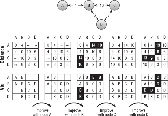
Figure 13-12: The shortest paths between all pairs of nodes in a network can be represented by a Distance array (top arrays) and a Via array (bottom arrays).

The upper-left array shows the initial values in the Distance array. The distance from each node to itself is 0. The distance between two nodes connected by a link is set to the link's cost. For example, the link between node A and node B has cost 4, so Distance[A, B] is 4. (To make the example easier to follow, the names of the nodes are used as if they were array indices.) The remaining entries are set to infinity.

The lower-left array shows the initial values in the Via array. For example, there is a link from node C to node B, so Via[C, B] is B.

After initializing the arrays, the algorithm looks for improvements. First it looks for paths it can improve by using node A as an intermediate point. Node A is on the end of the network, so it can't improve any paths.

Next the algorithm tries to improve paths by using node B and finds four improvements. For example, looking at the second Distance array, you can see that Distance[A, C] is infinity, but Distance[A, B] is 4 and Distance[B, C] is 10, so the path A → C can be improved. To make that improvement, the algorithm sets Distance[A, C] to 4 + 10 = 14 and sets Via[A, C] to the intermediate node B.

If you look at the network, you can follow the changes there. The initial path A→ C had distance set to infinity. The path A → B→ C is an improvement, and you can see in the network that the total distance for that path is 14.

Similarly you can work through the changes in the paths A → D, C → A, and D → A.

Next the algorithm tries to improve paths by using node C as an intermediate node. That node doesn't allow any improvements (because it's at the edge of the network).

Finally, the algorithm tries to improve paths by using node D as an intermediate node. It can use node D to improve the four paths A→ C, B → C, C → A, and C → B.

For an example of finding a path through the completed Via array, consider the array on the lower right in Figure 13-12. Suppose you want to find the path from node A to node C. The following steps describe how to find the path A → C:

• Via[A, C] is D, so A → C = A → D + D → C.
• Via[A, D] is B, so A → D = A → B + B → D.
• Via[D, C] is C, so there is a link from node D to node C.
• Via[A, B] is B, so there is a link from node A to node B.
• Finally, Via[B, D] is D, so there is a link from node B to node D.

The final path travels through nodes B, D, and C so the full path is A → B → D → C.

Figure 13-13 shows the recursive calls.

After you create the Distance and Via arrays, you can quickly find the shortest paths between any two points in a network. The downside is the arrays can take up a lot of room.

For example, a street network for a moderately large city might contain 30,000 nodes, so the arrays would contain 2 × 30,000² = 1.8 billion entries. If the entries are 4-byte integers, the arrays would occupy 7.2 gigabytes of memory.

Even if you can afford that much memory, the algorithm for building the arrays uses three nested loops that run from 1 to N, where N is the number of nodes, so the algorithm's total runtime is O(N³). If N is 30,000, that's 2.7 × 10¹³ steps. A computer running 1 million steps per second would need more than 10 months to build the arrays.

Figure 13-13: To find the path from start_node to end_node with intermediate point via_node, you recursively find the paths from start_node to via_node and from via_node to end_node.

For really big networks, this algorithm is impractical, so you need to use one of the other shortest-path algorithms to find paths as needed. If you need to find many paths on a smaller network, perhaps one with only a few hundred nodes, you may be able to use this algorithm to precompute all the shortest paths and save some time.

Summary

Most of the algorithms described in this chapter are traversals of networks. The depth-first and breadth-first traversal algorithms visit a network's nodes in different orders. The connectivity, spanning tree, minimal spanning tree, and shortest-path algorithms also all traverse the network in various ways. For example, the minimal spanning tree algorithm traverses links in order of their costs, and the label-setting shortest-path algorithm traverses links in order of the distances to their destination nodes.

The all-pairs shortest-path algorithm is a bit different. Instead of traversing the network, it builds a collection of N shortest-path trees, each of which lets you traverse the network.

The next chapter continues the discussion of networks. It explains more-advanced algorithms that let you solve real-world problems such as task ordering, map coloring, and work assignment.

Exercises

Asterisks indicate particularly difficult problems.

1. ^*Build a program similar to the one shown in Figure 13-14 that lets you build, save, and load test networks. Tools on the toolbar let the user add nodes, one-way links, and two-way links (actually two links connecting the clicked nodes in both directions). Give the File menu the commands New, Open, and Save As to let the user create, load, and save networks. (If you're using C# and don't want to build the whole program, you can download the example program from this book's website and replace the algorithmic code it contains with your own code.)

   

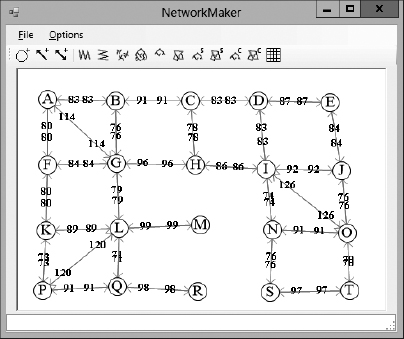
   Figure 13-14: The sample program NetworkMaker lets you build, save, and load test networks.

2. Expand the program you wrote for Exercise 1 to let the user traverse a network. If the user selects the traversal tool and then clicks a node, display a traversal of the nodes.
3. Expand the program you wrote for Exercise 1 to add a tool that displays the network's connected components.
4. Does the algorithm described for finding a network's connected components work for directed networks? Why or why not?
5. Expand the program you wrote for Exercise 1 to add a tool that finds and displays a spanning tree rooted at a node the user clicks.
6. The section “Minimal Spanning Trees” says that, in a network where every link has the same cost, every spanning tree is a minimal spanning tree. Why is that true?
7. Expand the program you wrote for Exercise 1 to add a tool that finds and displays a minimal spanning tree rooted at a node the user clicks.
8. Expand the program you wrote for Exercise 1 to add a tool that uses a spanning tree to find and display a path between two nodes the user selects.
9. Is a shortest-path tree always a minimal spanning tree? If so, why? If not, draw a counterexample.
10. Expand the program you wrote for Exercise 1 to add a tool that finds and displays a label-setting shortest-path tree rooted at a node the user clicks.
11. Expand the program you wrote for Exercise 1 to add a tool that uses a label-setting shortest-path tree to find and display a path between two nodes the user selects.
12. Expand the program you wrote for Exercise 1 to add a tool that finds and displays a label-correcting shortest-path tree rooted at a node the user clicks.
13. Expand the program you wrote for Exercise 1 to add a tool that uses a label-correcting shortest-path tree to find and display a path between two nodes the user selects.
14. What happens to the label-correcting shortest-path algorithm if the network contains a cycle that has a negative total weight? What happens to the label-setting algorithm?
15. Suppose you want to find the shortest path between two relatively close points in a large network. How could you make a label-setting algorithm find the path without building the entire shortest-path tree? Would the change save time?
16. ^*For the scenario in Exercise 15, how could you make a label-correcting algorithm find the path without building the entire shortest-path tree? Would the change save time?
17. ^*Suppose you're driving to a museum, and frequent road construction makes you leave the shortest path. After each change, you need to calculate a new shortest-path tree to find the best route from your new location to the museum. How could you avoid those recalculations?
18. ^*Expand the program you wrote for Exercise 1 to add a tool that finds and displays the Distance and Via arrays for a network. Verify the program on a network similar to the one shown in Figure 13-12.
19. ^*Expand the program you wrote for Exercise 18 so that the all-pairs shortest-path tool also displays the shortest paths between every pair of nodes in the network. Verify the program on a network similar to the one shown in Figure 13-12.
20. Assuming that your computer can execute 1 million steps per second while building the all-pairs shortest-path algorithm's Distance and Via arrays, how long would it take to build the arrays for a network with 100 nodes? 1,000 nodes? 10,000 nodes?
21. Using the network shown in Figure 13-15, draw the Distance and Via arrays as they evolve the same way Figure 13-13 does. What are the initial and final shortest paths from node A to node C?

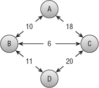
Figure 13-15: Draw the Distance and Via arrays for this network.