Chapter 2: Data Description and Simple Inference
2.2 Summary Statistics and Graphical Representations of Data
2.2.1 Initial Analysis of Room Width Guesses Using Simple Summary Statistics and Graphics
2.3 Testing Hypotheses and Student’s t-Test
2.3.1 Applying Student’s t-Test to the Guesses of Room Width
2.3.2 Checking the Assumptions Made When Using Student’s t-Test and Alternatives to the t-Test
2.4 The t-Test for Paired Data
2.4.1 Initial Analysis of Wave Energy Data Using Box Plots
2.4.2 Wave Power and Mooring Methods: Do Two Mooring Methods Differ in Bending Stress?
2.4.3 Checking the Assumptions of the Paired t-Tests
2.1 Introduction
In this chapter, we will describe how to get informative numerical summaries of data and graphs that allow us to assess various properties of the data. In addition, we will show how to test whether different populations have the same mean value for some variable of interest. The statistical topics covered are:
1. Summary statistics such as means and variances
2. Graphs such as histograms and box plots
3. Student’s t-test
2.2 Summary Statistics and Graphical Representations of Data
Shortly after metric units of length were officially introduced in Australia in the 1970s, each of a group of 44 students was asked to guess, to the nearest metre, the width of the lecture hall in which they were sitting. Another group of 69 students in the same room was asked to guess the width in feet, to the nearest foot. The measured width of the room was 13.1 metres (43.0 feet). The data were collected by Professor T. Lewis, and are given here in Table 2.1, which is taken from Hand et al. (1994). Of primary interest here is whether the guesses made in metres differ from the guesses made in feet, and which set of guesses gives the most accurate assessment of the true width of the room (accuracy in this context implies guesses that are closer to the measured width of the room).
Table 2.1: Room Width Estimates

2.2.1 Initial Analysis of Room Width Guesses Using Simple Summary Statistics and Graphics
How should we begin our investigation of the room width guesses data that are given in Table 2.1? As with most data sets, the initial data analysis steps should involve the calculation of simple summary statistics, such as means and variances, and graphs and diagrams that convey clearly the general characteristics of the data and perhaps enable any unusual observations or patterns in the data to be detected. The data set sasue.widths contains two variables: units and guess. First, we will convert the guesses made in metres into feet by multiplying them by 3.28 and then we will calculate the means and standard deviations of the metre and feet estimates.
To create a new variable with all estimates in feet, we will use a short program. A program tab is opened under Folders by clicking on the New button (![]() ) and selecting SAS program from the drop-down menu or by pressing F4. In the resulting program window, type and then run the following code;
) and selecting SAS program from the drop-down menu or by pressing F4. In the resulting program window, type and then run the following code;
data work.widths;
set sasue.widths;
if units='metres' then feet=guess*3.28;
else feet=guess;
run;
This creates a new version of the data set, work.widths, with a third variable, feet, which contains the guesses in feet. Data sets in the Work library are temporary in the sense that they are deleted when the session is finished.
Summary statistics can be produced using the SAS University Edition task of that name:
1. Open Tasks ▶ Statistics ▶ Summary Statistics.
2. Under Data ▶ Data, select work.widths.
3. Under Data ▶ Roles, select feet as the analysis variable and units as a Classification variable.
4. Click Run.
The edited results are shown in Output 2.1.
Output 2.1: Summary Statistics for Room Width Guesses Data
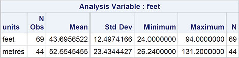
What do the summary statistics tell us about the two sets of guesses? It appears that the guesses made in feet are closer to the measured room width and less variable than the guesses made in metres, suggesting that the guesses made in the more familiar units, feet, are more accurate than those made in the recently introduced units, meters. But often such apparent differences in means and in variation can be traced to the effect of one or two unusual observations that statisticians like to call outliers. Such observations can usually be uncovered by some simple graphics, and here we shall construct box plots of the two sets of guesses after converting the guesses made in metres to feet.
A box plot is a graphical display useful for highlighting important distributional features of a continuous measurement. The diagram is based on what is known as the five-number summary of a data set, the numbers in question being the minimum, the lower quartile, the median, the upper quartile, and the maximum. The box plot is constructed by first drawing a box with ends at the lower and upper quartiles of the data; next, a horizontal line (or some other feature) is used to indicate the position of the median within the box and then lines are drawn from each end of the box to points defined by the upper quartile plus 1.5 times the interquartile range (the difference between the upper and lower quartiles) and the lower quartile minus 1.5 times the interquartile range. Any observations outside these limits are represented individually by some means in the finished graphic, and such observations are likely candidates to be labelled outliers. The resulting diagram schematically represents the body of the data minus the extreme observations and is particularly useful for comparing the distributional features of a measurement made in different groups.
The Summary Statistics task also produces box plots (under options ▶ Plots ▶ Comparative box plot), but this does not display outliers in the way described above. Instead, we will use the Box Plot task:
1. Open Tasks ▶ Graph ▶ Box Plot.
2. Under Data ▶ Data, select work.widths.
3. Under Data ▶ Roles, add feet as the Analysis variable and units as the Category variable.
4. Click Run.
The resulting plots are shown in Figure 2.1; they indicate that both sets of guesses contain a number of possible outliers and also that the guesses made in metres are skewed (have a longer tail) and are more variable than the guesses made in feet. We shall return to these findings in the next subsection.
Figure 2.1: Box Plots of Room Width Guesses Made in Feet and in Metres (After Conversion to Feet)
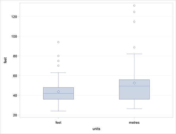
Box plots are our favourite graphic for comparing the distributional properties of a measurement made in different groups, and they are available as optional plots in several of the statistical tasks. Another graphic for displaying distributions is the histogram. In a histogram, the range of values is divided into small intervals and the number of observations within each interval is represented by the area of a rectangle centred on the interval; if intervals are all equal, then the heights of the rectangles are proportional to the observed frequencies.
The Histogram task within Tasks ▶ Graph can be used to produce a single histogram. For a comparative histogram, we will use the Distribution Analysis task within Tasks ▶ Statistics:
1. Open Tasks ▶ Statistics ▶ Distribution Analysis.
2. Under Data ▶ Data, select work.widths.
3. Under Data ▶ Roles, add feet as the Analysis variable.
4. Under Options ▶ Exploring data ▶ Histogram ▶ Classification Variables, add units.
5. Click Run.
The resulting plots are shown in Figure 2.2; they show clearly the greater skewness in the guesses made in metres.
Figure 2.2: Histograms for Room Width Guesses Data

2.3 Testing Hypotheses and Student’s t-Test
From the summary statistics and graphics produced in the previous subsection, we already know quite a bit about how the guesses of room width made in feet differ from the guesses made in metres. The guesses made in feet appear to be concentrated around the measured room width of 43.0 feet, whereas the guesses made in meters suggest overestimation of the width of the room. In some circumstances, we might simply stop here and try to find an explanation of the apparent difference between the two types of guesses (and many statisticians would be sympathetic to this approach!). But, in general, the investigation of the data will need to go further and use more formal statistical methods to try to confirm our very strong hunch that guesses of room width made in metres differ from guesses made in feet.
The area of statistics that we need to move into is that of statistical inference, the process of drawing conclusions about a population on the basis of measurements or observations made on a sample of observations from the population, a process that is central to statistics. More specifically, inference is about testing hypotheses of interest about some population value on the basis of the sample values, and involves what is known as significance tests. For the room width guesses data in Table 2.1, for example, there are three hypotheses that we might wish to test:
In the population of guesses made in metres, the mean is the same as the true room width (namely, 13.1 metres). Formally, we might write this hypothesis as
where H0 denotes the null hypothesis.
In the population of guesses made in feet, the mean is the same as the true room width (namely, 43.0 feet), that is
H0 : μf = 43.0
After the conversion of metres into feet, the population means of both types of guess are equal, or in formal terms
H0 : μmx3.28 = μf
(It might be imagined that a conclusion about the last of these three hypotheses would be implied from the results found for the first two, but as we shall see later this is not the case.)
2.3.1 Applying Student’s t-Test to the Guesses of Room Width
Testing hypotheses about population means requires what is known as the Student’s t-test. The test is described in detail in Altman (1991) but in essence involves the calculation of a test statistic from sample means and standard deviations, the distribution of which is known if the null hypothesis is true and certain assumptions are met. From the known distribution of the test statistic, a p-value can be found.
The p-value is probably the most ubiquitous statistical index found in the applied sciences literature and is particularly widely used in biomedical and psychological research. So just what is the p-value? Well, the p-value is the probability of obtaining the observed data (or data that represent a more extreme departure from the null hypothesis) if the null hypothesis is true. It was first proposed as part of a quasi-formal method of inference by a famous statistician, Ronald Aylmer Fisher, in his influential 1925 book, Statistical Methods for Research Workers. For Fisher, the p-value represented an attempt to provide a relatively informal measure of evidence against the null hypothesis; the smaller the p-value, the greater the evidence that the null hypothesis is incorrect.
But, sadly, Fisher’s informal approach to interpreting the p-value has long ago been abandoned in favour of a simple division of results into significant and non-significant on the basis of comparing the p-value with some largely arbitrary threshold value such as 0.05. The implication of this division is that there can always be a simple yes (significant) or no (non-significant) answer as the fundamental result from a study; this is clearly false, and used in this way hypothesis testing is of limited value.
In fact, overemphasis on hypothesis testing and the use of p-values to dichotomise significant or non-significant results has distracted from other more useful approaches to interpreting study results, in particular the use of confidence intervals. Such intervals are a far more useful alternative to p-values for presenting results in relation to a statistical null hypothesis and give a range of values for a quantity of interest that includes the population value of the quantity with some specified probability. (Confidence intervals are described in detail in Altman, 1991.) In essence, the significance test and associated p-value relate to what the population quantity of interest is not; the confidence interval gives a plausible range for what the quantity is.
So, after this rather lengthy digression, let’s apply the relevant Student’s t-tests to the three hypotheses that we are interested in assessing on the room width data. The first two hypotheses require the application of the single sample t-test, referred to in the software as a one-sample t-test, separately to each set of guesses. We start by splitting the widths data set into two parts according to whether the guesses were made in metres or feet:
1. Open Tasks ▶ Data ▶ Filter Data.
2. Under Data ▶ Data, add work.widths.
3. Under Data ▶ Filter, assign units as variable 1, set the comparison to Equal, and type feet in the Value box.
4. Under Data ▶ Output Data Set, type feet.
5. Click Run.
The result is a temporary data set, feet, in the Work library. Repeat the above, entering metres instead of feet in steps 3 and 4 (above). Then, to apply the single sample t-test to the guesses in feet:
1. Open Tasks ▶ Statistics ▶ T Tests.
2. Under Data ▶ Data, add work.feet.
3. Under Data ▶ Roles ▶ Analysis variable, add guess. Note that One-sample test is the default.
4. Under Options ▶ Tests ▶ Alternative hypothesis, enter 43 in the box and deselect Tests for normality.
5. Click Run.
For the guesses made in metres, repeat the above using work.metres in step 2 and 13.1 for the value in step 4.
The results are shown in Output 2.2. Let’s now look at these results in some detail. Looking first at the two p-values, we see that there is no evidence that the guesses made in feet differ in mean from the true width of the room, 43 feet (the 95% confidence interval here is [40.69, 46.70] feet, which includes the true value of 43 feet). But there is considerable evidence that the guesses made in metres do differ from the true value of 13.1 metres; here, the confidence interval is [13.85, 18.20] and the students appear to systematically overestimate the width of the room when guessing in metres.
Output 2.2: Results of Single Sample t-Tests for Room Width Guesses Made in Feet and for Guesses Made in Metres
a) Guesses Made in Feet


b) Guesses Made in Metres

Now it might be thought that our third hypothesis discussed above, namely that the mean of the guesses made in feet and the mean of the guesses made in metres (after conversion to feet) are the same, can be assessed simply from the results given in Output 2.2. Because the population mean of guesses made in feet apparently does not differ from the true width of the lecture room, but the population mean of guesses does differ from the true value, then surely the means of the two groups of guesses differ from each other? Not necessarily, and to assess the equality of means hypothesis correctly, we need to apply an independent samples t-test to the data. We again use the t-test task:
1. Open Tasks ▶ Statistics ▶ T Test.
2. Under Data ▶ Data, add work.widths.
3. Under Data ▶ Roles ▶ T test, select Two-sample test.
4. Under Data ▶ Roles ▶ Analysis variable, add feet as the Analysis variable and units as the Groups variable.
5. Click Run.
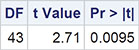
The results of applying this test are shown in Output 2.3. (The graphical output shown in Figures 2.3 (a) and (b) will be discussed in the next subsection.) Ignoring for the moment the tests for normality, we look first at the p-value associated with the t-test when equality of variances is assumed; the value is p=0.0102, from which we can conclude that there is considerable evidence that the population means of the two types of guesses do indeed differ. The confidence interval for the difference [-15.57,-2.15] indicates that the guesses made in feet have a mean that is between about 15 and 2 feet lower than the guesses made in metres.
Output 2.3: Results of Applying Independent Samples t-Test to the Room Width Guesses Data


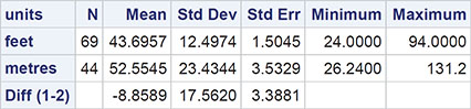


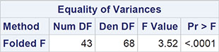
Figure 2.3 (a): Histograms of Length Guesses in Feet and in Meters After Conversion to Feet with Fitted Normal Distributions and Kernel Density Function Estimates

Figure 2.3 (b): Probability Plots of Length Guesses

2.3.2 Checking the Assumptions Made When Using Student’s t-Test and Alternatives to the t-Test
Having applied t-tests to assess each of the hypotheses of interest and having found the corresponding p-values and confidence intervals, it might appear that we have finished the analysis of the room width data. But as yet, we have not looked at the assumptions that underlie the t-tests and have not checked whether these assumptions are likely to be valid for the data. First the assumptions:
• The measurements are assumed to be sampled from a normal distribution.
• For the independent samples t-test, each population is assumed to have the same variance.
• The measurements made are independent of each other.
If any (or all) of these assumptions is invalid, then strictly speaking, the t-test is also not valid. In practice small departures from the assumptions are unlikely to be of any great importance, but it is still worth trying (at least informally) to check whether the data meet the assumptions. So first let’s consider the normality assumption. The results of applying a number of formal tests of normality are shown in Output 2.3. Each of these tests is described in detail in Everitt and Skrondal (2010); they are all highly significant, indicating that the normality assumption is in doubt for length guesses both in feet and in meters. But these formal tests can often be misleading and are rarely used.
Preferable for checking the normality assumption is to use histograms of the data enhanced by fitted normal distributions as shown in Figure 2.3 (a) (the kernel estimate shown in the plot is explained in Der and Everitt, 2013; it is essentially a method of estimating a distribution without assuming any specified distributional form, for example a normal distribution) and what is known as a probability plot, which in essence involves a plot of the observed quantiles against theoretical quantiles of the normal distribution (for details, see Everitt and Palmer, 2005). Such plots should have the form of a straight line, that is, they should be linear, if the sample does arise from a normal distribution. These plots are shown in Figure 2.3 (b).
Both graphics, but particularly those for the guesses in metres, throw the normality assumption required for the t-test to be valid into some doubt. This possible non-normality combined with the evidence that two types of guesses have different variances obtained from both the initial examination of the data and the test for equality of variances (see Altman, 1991) given in Output 2.3 suggests that some caution is needed in interpreting the results from our t-tests. Fortunately, the t-test is known to be relatively robust against departures both from normality and the homogeneity assumption, although it is somewhat difficult to predict how a combination of non-normality, heterogeneity, and outliers will affect the test.
Since the test for equality of variance given in Output 2.3 has an associated p-value of <0.001, we should perhaps first consider using a modified version of the t-test in which the equality of variance assumption is dropped (see Altman, 1991, for details). The p-value of the modified test (Satterthwaite test-see Everitt and Skrondal, 2010) is also given in Output 2.3 and, although less significant than the usual form of the t-test, still shows evidence for a difference in the population means of the two types of room width guesses.
Here, however, given the existence of outliers in the data and their possible non-normality, we might ask whether an alternative test is available that is both insensitive to the effect of outliers and does not assume normality.
An alternative to Student’s t-test that does not depend on the assumption of normality is the Wilcoxon Mann-Whitney test; this test, which since it is based on the ranks of the observations, is also unlikely to be affected greatly by outliers. The Wilcoxon Mann-Whitney test, which is described in detail in Altman (1991), assesses whether the distribution of the measurements in the two groups is the same. This is available in the t-test task and is applied as follows: reopen the t-tests task or repeat steps 1 to 4 above:
1. Under Options ▶ Tests, select Wilcoxon rank-sum test.
2. Click Run.
The p-value for the test is 0.028, confirming the difference in location between the guesses in feet and the guesses in metres.
2.4 The t-Test for Paired Data
In a design study for a device to generate electricity from wave power at sea, experiments were carried out on scale models in a wave tank to establish how the choice of mooring method for the system affected the bending stress produced in part of the device. The wave tank could simulate a wide range of sea states (rough, calm, moderate, and so on), and the model system was subjected to the same sample of sea states with each of two mooring methods, one of which was considerably cheaper than the other. The resulting data giving root mean square bending moment in Newton metres are shown in Table 2.2 (these data are taken from Hand et al., 1994). The question of interest is whether bending stress differs for the two mooring methods.
Table 2.2: Wave Energy Device Mooring Data

2.4.1 Initial Analysis of Wave Energy Data Using Box Plots
For the wave energy data in Table 2.2, we will construct box plots of the bending stresses for each mooring method and here, for reasons that will become apparent in the next subsection, it is also useful to have a look at the box plot of the differences between the pairs of observations made for the same sea state.
The dataset sasue.waves contains variables: state, method1, method2, and difference.
1. Open Tasks ▶ Data ▶ Transform data.
2. Graph ▶ Box Plot
3. Click Run.
Run the box plot task twice more, once each with method2 and difference as the analysis variable. The results are shown in Figures 2.4 (a), (b) and (c).
Figure 2.4: Box Plots of Root Mean Square Bending Moment (Newton Metres) for Mooring Methods I and II
(a) Method I

(b) Method II
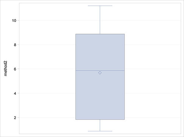
Figure 2.5: Box Plot of Differences of Root Mean Square Bending Moment for the Two Mooring Methods
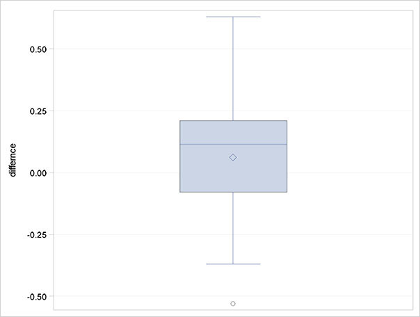
The box plot of differences in Figure 2.5 suggests that there might be one outlying observation that we might wish to check, and a small degree of skewness, although with only 18 observations, drawing any conclusions about the distributional properties of the data is difficult.
2.4.2 Wave Power and Mooring Methods: Do Two Mooring Methods Differ in Bending Stress?
Now we can move on to consider more formally the questions of interest about the wave energy data. Superficially, these data look to be of a very similar format to the room width guesses data, but closer consideration shows that there is a fundamental difference in that the observations are paired; that is, the bending stress for each of the two mooring methods is, in each case, based on the same sea state. Consequently, these observations are likely to be correlated rather than independent. So here to test whether there is a difference in the mean bending stress of the two methods of mooring, we use what is called a paired t-test (see Altman, 1991, for details); essentially, this test is the same as the one-sample t-test used previously for the room width data, but here the null hypothesis is that the population mean of the differences of the paired observations is zero. To apply the test:
1. Open Tasks ▶ Statistics ▶ T Tests.
2. Under Data ▶ Data, add sasue.waves.
3. Under Data ▶ Roles ▶ T Test, choose Paired test.
4. Under Data ▶ Roles, select method1 as the Group 1 variable and method2 as the Group2 variable.
5. Under Options ▶ Tests, deselect Tests for normality.
6. Under Options ▶ Plots, choose selected plots and select Histogram and box plot.
7. Run.
The salient numerical results are shown in Output 2.4. The p-value associated with the paired t-test applied to the wave power data is 0.38. There is no evidence of a difference in mean bending stress for the two mooring methods. The associated graphic in Figure 2.6 indicates that the normality assumption for the differences is justified.
Output 2.4: Results of Applying the Paired t-Test to the Wave Power Data
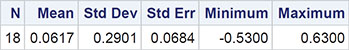
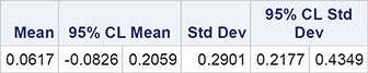
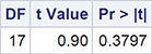
Figure 2.6: Histogram and Fitted Normal Distribution for the Differences in Bending Stress of the Two Mooring Methods

2.4.3 Checking the Assumptions of the Paired t-Tests
For the paired t-test to be valid, the differences between the paired observations need to be normally distributed. We could use a probability plot to assess the required normality of the differences, but with only 18 observations for the wave data, the plot would not be very useful. Since we cannot satisfactorily assess the normality assumption for these data, we might wish to consider a non-parametric alternative; this would be the Wilcoxon signed rank test.
The non-parametric analogue of the paired t-test is Wilcoxon’s signed rank test (see Altman, 1991, for details). As with the Wilcoxon Mann-Whitney test described above, the signed rank test uses only the ranks of the observations and does not assume normality for the observations; the test is available as an option for the t-Tests task:
1. Reopen the T tests task or repeat steps 1 to 6 above.
2. Under Options ▶ Tests, select Sign test and Wilcoxon signed rank test.
3. Click Run.
This is also an alternative way of applying a matched-pairs t-test, as can be seen from the results in Output 2.5.
Output 2.5: Wilcoxon Signed Rank Test for Wave Energy Mooring Data
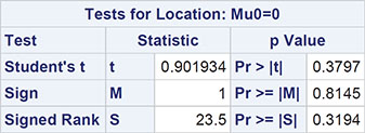
The test gives a p-value of 0.319, confirming the result from the paired t-test.
2.5 Exercises
Exercise 2.1: Babies Data
The data set, babies, gives the recorded birth weights of 50 infants who displayed severe idiopathic respiratory distress syndrome (SIRDS). SIRDS is a serious condition that can result in death and did so in the case of 27 of these children. One of the questions of interest about these data is whether the babies who died differed in birth weight from the babies who survived. Use some suitable graphical techniques to carry out an initial analysis of these data and then find a 95% confidence interval for the difference in mean birth weight for SIRDS babies who die and SIRDS babies who live.
Birth Weights (kg)

Exercise 2.2: Choles Data
The data in the choles data set were collected by the Western Collaborative Group Study carried out in California in 1960-1961. In this study, 3,154 middle-aged men were used to investigate the possible relationship between behaviour pattern and risk of coronary heart disease. The data set contains data from the 38 heaviest men in the study (all weighing at least 225 pounds). Cholesterol measurements (mg/100ml) and behaviour type were recorded; type A behaviour is characterized by urgency, aggression, and ambition, and type B behaviour is relaxed, non-competitive, and less hurried. The question of interest is whether, in heavy middle-aged men, cholesterol level is related to behaviour type. Investigate the question of interest in any way that you feel is appropriate, paying particular attention to assumptions and to any observations that might possibly distort conclusions.
Type A:
233 291 312 250 246 197 268 224 329 239 254 276 234 181 248 252 202 218 325
Type B:
420 185 263 246 224 212 188 250 148 169 226 175 242 153 183 137 202 194 213
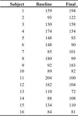
Exercise 2.3: Diet Data
The data in diet come from a study of the Stillman diet, a diet that consists primarily of protein and animal fats and that restricts carbohydrate intake. In diet, triglyceride values (mg/100ml) are given for 16 participants both before beginning the diet and at the end of a period of time following the diet. Here interest is on whether there has been a change in triglyceride level that might be attributed to the diet. Carry out an appropriate hypothesis test to investigate whether there has been a change in triglyceride level, using any graphics that you think might be helpful in interpreting the test.