
Chapter 8: Poisson Regression and the Generalized Linear Model
8.2.1 Components of Generalized Linear Models
8.2.2 Using the Generalized Linear Model to Apply Multiple Linear Regression and Logistic Regression
8.3.1 Example 1: Familial Adenomatous Polyposis (FAP)
8.3.2 Example 2: Bladder Cancer
8.1 Introduction
In this chapter, we show how the multiple linear regression model and the logistic regression model can both be subsumed within a more general modelling framework, the generalized linear model (GLM), and how the GLM then leads to more appropriate models for response variables that cannot (and should not) be modelled by the methods described in either Chapter 6 or Chapter 7. The statistical topics to be covered are
• Generalized linear model
• Linear and logistic regression fitted using the generalized linear model
• Poisson regression
8.2 Generalized Linear Model
The term generalized linear model (GLM) was first introduced in a landmark paper by Nelder and Wedderburn (1972), in which a wide range of seemingly disparate problems of statistical modeling and inference were set in an elegant, unifying framework of great power and flexibility. Generalized linear models include all the modeling techniques described in earlier chapters (that is analysis of variance, analysis of covariance, multiple linear regression, and logistic regression) and open up the possibility of other models--for example, Poisson regression, which we shall describe in this chapter. A comprehensive account of GLMs is given in McCullagh and Nelder (1989) and a more concise and less technical description in Dobson and Barnett (2008). In the next subsection, we very briefly review the main features of such models.
8.2.1 Components of Generalized Linear Models
The multiple linear regression model described in Chapter 6 has the form
The error term, ε, is assumed to have a normal distribution with zero mean and constant variance, σ2. An equivalent way of writing the model is as y ~ N(μ,σ2) where μ = β0 + β1x1 + ... + βqxq. This makes it clear that this model is only suitable for continuous response variables with, conditional on the values of the explanatory variables, a normal distribution with constant variance. The generalization of such a model made in GLMs consists of allowing each of the following three assumptions associated with the multiple linear regression model to be modified:
• The response variable is normally distributed with a mean determined by the model.
• The mean can be modelled as a linear function (possibly nonlinear transformations) of the explanatory variables (that is, the effects of the explanatory variables on the mean are additive).
• The variance of the response variable, given the (predicted) mean, is constant.
In a GLM, some transformation of the mean is modelled by a linear function of the explanatory variables, and the distribution of the response variable around its mean (often referred to as the error distribution) is generalized, usually in a way that fits naturally with a particular transformation. (We shall deal with the last bullet point above later in the chapter.) The result is a very wide class of regression models that includes many other models as special cases (for example, analysis of variance, multiple linear regression, and logistic regression). The three essential components of a GLM are
1. A linear predictor, η, formed from the explanatory variables:
η = β0 + β1x1 + β2x2 ... + βqxq
2. A transformation of the mean, μ, of the response variable called the link function, g(μ. In a GLM, it is g(μ), which is modelled by the linear predictor:
g(μ)=η
In multiple linear regression and analysis of variance, the link function is the identity function so that the mean is modelled directly as a linear function of the explanatory variables. In logistic regression, the link function is the logit--that is, the log of the odds ratio is modelled.
3. The distribution of the response variable given its mean μ is assumed to be of some particular type from a family of distributions known as the exponential family; for details, see Dobson and Barnett (2008).
The parameters in GLMs are estimated by maximizing the joint likelihood of the observed responses given the parameters of the model and the explanatory variables. This generally requires iterative numerical algorithms. See McCullagh and Nelder (1989) for details.
8.2.2 Using the Generalized Linear Model to Apply Multiple Linear Regression and Logistic Regression
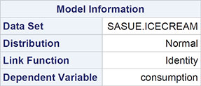
Here we will illustrate how two sets of data, the ice cream consumption data used in Chapter 6 and the survival from surgery data that appeared in Chapter 7, can be analysed by applying the same models used in those two previous chapters within a generalized linear modelling framework.
So, first the ice cream consumption data where the SAS University Edition code now is:
1. Open Tasks ▶ Statistics ▶ Generalized Linear Models.
2. Under Data ▶ Data, select sasue.icecream.
3. Under Data ▶ Roles ▶ Response ▶ Distribution, select normal and add consumption as the response variable.
4. Under Data ▶ Roles ▶ Explanatory Variables ▶ Continuous Variables, add price and temperature.
5. Under Model ▶ Model Effects, add price and temperature.
6. Click Run.
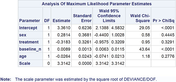
The edited output is shown in Output 8.1. The first part of the output identifies the data set, the distribution assumed, and the link function. The next part lists the values of a number of goodness-of-fit indicators. Some of these, such as the AIC and AICC, have been briefly discussed in Chapter 6; the BIC, standing for Bayesian information criterion, is similar to the AIC, but penalizes models of high dimensionality more than that index. The deviance we will explain later in the chapter. The parameter estimates are found next, and these are the same as those given in Chapter 6. The scale parameter mentioned will be explained in Section 8.4. The Wald statistic is simply the ratio of an estimated parameter to its estimated standard error. Under the hypothesis that the population parameter value is 0, the square of the Wald statistic has a chi-square distribution with a single degree of freedom.
Output 8.1: Edited Output from Applying Generalized Linear Modelling to the Ice Cream Consumption Data


Algorithm converged.

Now we can move on to the analysis of the survival for surgery data, where the logistic regression model described in Chapter 7 can be fitted within the generalized linear model framework as follows:
1. Open Tasks ▶ Statistics ▶ Generalized Linear Models.
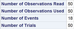
2. Under Data ▶ Data, select sasue.sepsis.
3. Under Data ▶ Roles ▶ Response ▶ Distribution, select Binomial, add survival as the response variable, and select Higher value as the event of interest.
4. Under Data ▶ Roles ▶ Explanatory Variables ▶ Continuous Variables, add all the remaining variables except ID.
5. Under Model ▶ Model Effects, add all the variables.
6. Click Run.
The edited output is shown in Output 8.2. Here the first part of the output details that the distribution assumption is binomial and the link is the logit function, giving the logistic regression model. The parameter estimates are the same as those given in Output 7.4 of Chapter 7. Again, the scale function mentioned will be discussed later.
Output 8.2: Edited Output from Applying the Generalized Linear Model to the Survival from Surgery Data
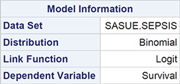

PROC GENMOD is modeling the probability that Survival='1'.

Algorithm converged.
8.3 Poisson Regression
The Poisson regression model is useful for a response variable, y, that is a count or frequency and for which it is reasonable to assume an underlying Poisson distribution, that is:
In Poisson regression, it is the log of the response variable’s mean that is modelled as a linear function of the explanatory variables. In other words, in the GLM framework, the link function is the log function and the error distribution is Poisson. The log link is needed to prevent any predicted values of the response variable being negative.
8.3.1 Example 1: Familial Adenomatous Polyposis (FAP)
As an example of Poisson regression, we shall apply the method to the data shown in Table 8.1 taken from Piantadosi (1997). The data arise from a study of Familial Adenomatous Polyposis (FAP), an autosomal dominant genetic defect that predisposes those affected to develop large numbers of polyps in the colon, which, if untreated, could develop into colon cancer. Patients with FAP were randomly assigned to receive an active drug treatment or a placebo. The response variable was the number of colonic polyps at 3 months after starting treatment. Additional covariates of interest were the number of polyps before starting treatment, gender, and age.
Table 8.1: FAP Data

Treatment: 0=placebo, 1=active
A Poisson regression model can be fitted as follows:
1. Open Tasks ▶ Statistics ▶ Generalized Linear Models.
2. Under Data ▶ Data, select sasue.fap.
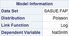
3. Under Data ▶ Roles ▶ Response ▶ Distribution, select Poisson and add Nat3mth as the response variable.
4. Under Data ▶ Roles ▶ Explanatory Variables ▶ Continuous Variables, add all the remaining variables.
5. Under Model ▶ Model Effects, add all the variables.
6. Click Run.
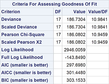
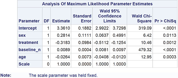
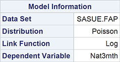
The numerical results are shown in Output 8.3. The regression coefficients become easier to interpret if they (and the confidence limits) are exponentiated. For example, the exponentiated confidence interval for the gender regression coefficient is [1.066, 1.647]; men are estimated to have somewhere between about 7% and 65% more polyps at 3 months than women, conditional on the other covariates being the same. For treatment, the corresponding interval is [0.600, 0.882]; patients receiving the active treatment are estimated to have between 60% and 88% of the number of polyps at 3 months than those receiving the placebo, again conditional on the other covariates being equal.
Here we should say something about the deviance term in Output 8.3 and previous output in this chapter. This is essentially a measure of how a model fits the data and is most useful in comparing two competing nested models (that is, two models in which one contains terms that are additional to those in the other). The difference in deviance between two nested models measures the extent to which the additional terms improve the fit of the more complex model. The difference in deviance has approximately a chi-square distribution with degrees of freedom equal to the difference in the degrees of freedom of the two nested models. Exercise 8.3 gives an opportunity for readers to investigate using the deviance in this way.
(For the multiple regression model, a generalized linear model with a normal distribution and an identity link function, the deviance is simply the residual sum of squares from the usual analysis of variance table for such a model. See Chapter 6 for more information.)
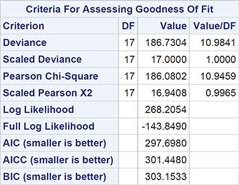
It should be noted that one aspect of the fitted Poisson regression model to the FAP data, namely the value of the deviance divided by the degrees of freedom (the value 10.98 in Output 8.3) has implications for the appropriateness of the model, a point we shall take up in detail in the next section.
Output 8.3: Numerical Output from Fitting Poisson Regression to the FAP Data

Algorithm converged.
8.3.2 Example 2: Bladder Cancer
As a further example of the use of Poisson regression, we shall use the data shown in Table 8.2, taken from Seeber (1989). The data arise from 31 male patients who have been treated for superficial bladder cancer. They give the number of recurrent tumours during a particular time period after removal of the primary tumour and the size of the primary tumour (whether smaller or larger than 3 cm).
Table 8.2: Bladder Cancer Data (Used with Permission of the Publishers, John Wiley and Sons Ltd, from Seeber, 1998)
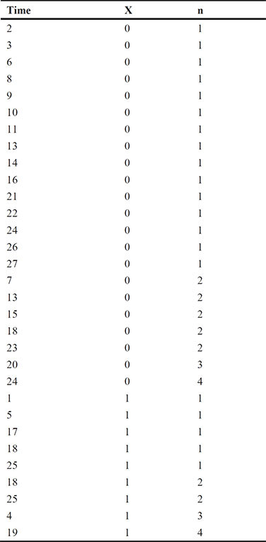
X = 0 tumour < 3 cm
X = 1 tumour > 3 cm
Before coming to the analysis of the data in Table 8.2, we first need to introduce the idea of a Poisson process, in which the waiting times between successive events of interest (the tumours, in this case) are independent and exponentially distributed with a common mean, 1λ (say). Then, the number of events that occur up to time t has a Poisson distribution with mean μ = λt. Here the parameter of real interest is the rate at which events occur, λ, and for a single explanatory variable, x, we can adopt a Poisson regression approach using the following model to examine the dependence of λ on x:
Rearranging this model, we obtain
In this form, the model can be fitted within the GLM framework with a log link and Poisson errors. But in this model log t is a variable in the model whose regression coefficient is fixed at unity and is usually known as an offset. To create the offset variable, we first transform the time variable to log_time using the Transform Data task as follows:
1. Open Tasks ▶ Data ▶ Transform Data.
2. Under Data ▶ Data, select sasue.bladder.
3. Under Data ▶ Transform 1 ▶ Variable 1, add time and select Natural Log as the transform.
4. Under Data ▶ Output Data Set, delete Transform and type sasue.bladder.
5. Click Run.
The Poisson regression model is fitted to the bladder cancer data as follows:
1. Open Tasks ▶ Statistics ▶ Generalized Linear Models.
2. Under Data ▶ Data, select sasue.bladder.
3. Under Data ▶ Roles ▶ Response ▶ Distribution, select Poisson and add n as the response variable.
4. Under Data ▶ Roles ▶ Explanatory Variables ▶ Continuous Variables, add x.
5. Under Data ▶ Roles ▶ Explanatory Variables ▶ Offset Variable, add log_time.
6. Under Model ▶ Model Effects, add x. The offset, log_time, is added automatically.
7. Click Run.
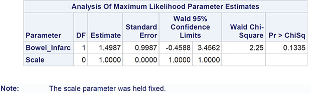
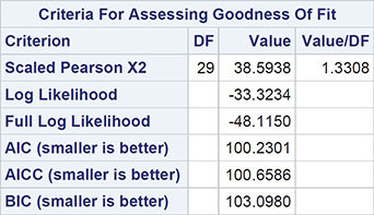
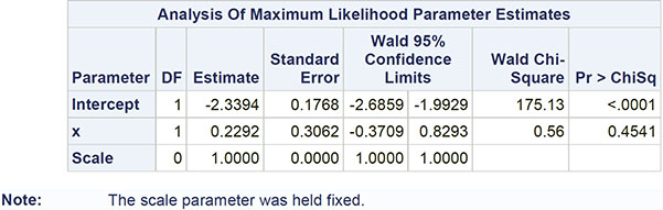
The numerical results are shown in Output 8.4. The estimated model is
log λ = −2.339 + 0.229x
So, for smaller tumors (x=0), the estimated (baseline) rate is exp(-2.339)=0.096, and for larger tumors (x=1), the estimated rate is exp(-2.339+0.229)=0.12. The rate for larger tumors is estimated as 0.12/0.096=1.25 times the rate for smaller tumours. In terms of waiting times between recurrences, the means are 1/0.096=10.42 months for smaller tumours and 1/0.12=8.33 months for larger tumors. But the regression coefficient for the dummy variable that codes for tumour size is seen from Output 8.4 to be non-significant, so the data give no evidence that rates or waiting times for large and small tumours are different. This becomes apparent if we construct a confidence interval for the rate for larger tumours from the confidence limits given in Output 8.4 as [exp(-2.339-0.371), exp(-2.339+0.829)], that is [0.067, 0.221]. This interval contains the rate for smaller tumours. There is no evidence that the size of the primary tumour is associated with the number of recurrent tumours.
Output 8.4: Numerical Results from Fitting the Poisson Regression Model to the Bladder Cancer Data


Algorithm converged.
8.4 Overdispersion
An important aspect of generalized linear models that thus far we have largely ignored is the variance function, V(μ), that captures how the variance of a response variable depends on its mean. The general form of the relationship is Var(response)=φV(μ), where φ is a constant and V(μ) specifies how the variance depends on the mean, μ. For the error distributions considered previously, this general form becomes
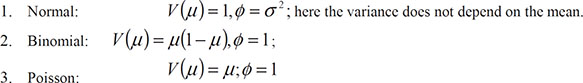
In the case of a Poisson variable, we see that the mean and variance are equal, and in the case of a binomial variable where the mean is the probability of the occurrence of the event of interest, p, the variance is p(1 − p).
Both the Poisson and binomial distributions have variance functions that are completely determined by the mean. There is no free parameter for the variance because in applications of the generalized linear model with binomial or Poisson error distributions, the dispersion parameter, φ, is defined as 1 (see previous results for logistic and Poisson regression). But in some applications, this becomes too restrictive to fully account for the empirical variance in the data; in such cases, it is common to describe the phenomenon as overdispersion. For example, if the response variable is the proportion of family members who have been ill in the past year, observed in a large number of families, then the individual binary observations that make up the observed proportions are likely to be correlated rather than independent. This non-independence can lead to a variance that is greater (less) than that on the assumption of binomial variability. And observed counts often exhibit larger variance than would be expected from the Poisson assumption, a fact noted by Greenwood and Yule over 80 years ago (Greenwood and Yule, 1920). Greenwood and Yule’s suggested solution to the problem was a model in which μ was a random variable with a gamma distribution leading to a negative binomial distribution for the count.
There are a number of strategies for accommodating overdispersion, but here we concentrate on a relatively simple approach that retains the use of the binomial or Poisson error distributions as appropriate but allows estimation of a value of φ from the data rather than defining it to be unity for these distributions. The estimate is usually the residual deviance divided by its degrees of freedom, exactly the method used with Gaussian models. Parameter estimates remain the same, but parameter standard errors are increased by multiplying them by the square root of the estimated dispersion parameter. This process can be carried out manually, or almost equivalently the overdispersed model can be formally fitted using a procedure known as quasi-likelihood. This allows estimation of model parameters without fully knowing the error distribution of the response variable. See McCullagh and Nelder (1989) for full technical details on this approach.
When fitting generalized linear models with binomial or Poisson error distributions, overdisperson can often be spotted by comparing the residual deviance with its degrees of freedom. For a well-fitting model, the two quantities should be approximately equal. If the deviance is far greater than the degrees of freedom, overdispersion might be indicated. In Output 8.3, for example, we see that the ratio of deviance to degrees of freedom is nearly 11, clearly indicating an overdispersion problem. Consequently, we will now refit the Poisson model with the square root of the deviance divided by its degrees of freedom as the scale parameter using the following codeL
1. Open Tasks ▶ Statistics ▶ Generalized Linear Models.
2. Under Data ▶ Data, select sasue.fap.
3. Under Data ▶ Roles ▶ Response ▶ Distribution, select Poisson and add Nat3mth as the response variable.
4. Under Data ▶ Roles ▶ Explanatory Variables ▶ Continuous Variables, add all the remaining variables.
5. Under Model ▶ Model Effects, add all the variables.
6. Under Options ▶ Methods ▶ Dispersion, select Adjust for dispersion and from the drop-down menu, select Use deviance estimate.
7. Click Run.
Output 8.5: Numeric Results of Fitting Overdispersed Poisson Model to FAP Data

Algorithm converged.
The results are shown in Output 8.5. Comparing these with the results in Output 8.3, we see that the estimated regression coefficients are the same, but their standard errors are now much greater, with the consequence that only the coefficient of the baseline polyps count remains significant. Gender, treatment, and age are no longer found to be significant predictors of 3-month polyp count.
For a more detailed discussion of overdispersion, see Collett (2003).
8.5 Summary
Generalized linear models provide a very powerful and flexible framework for the application of regression models to medical data. Some familiarity with the basis of such models may allow medical researchers to consider more realistic models for their data rather than relying solely on linear and logistic regression.
8.6 Exercises
Exercise 8.1: Coronary Heart Disease Data
The data in the chd data set arise from a prospective study of potential risk factors for coronary heart disease (CHD) (Rosenman et al., 1975). The study looked at 3,154 men aged 40-50 for an average of 8 years and recorded the incidence of cases of CHD. The potential risk factors included smoking, blood pressure, and personality/behavior type.
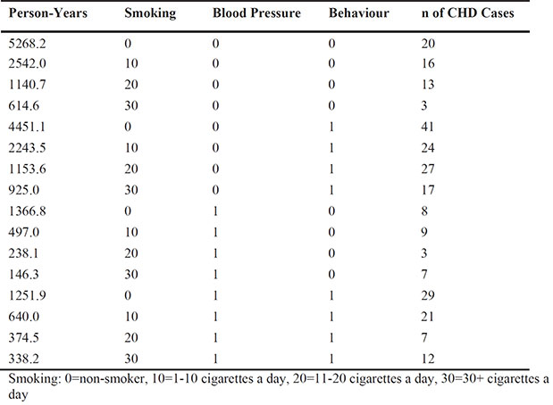
Blood pressure: 0=<140, 1=≥140
Behaviour: 0=Type B personality,1=Type A personality (Type A are characterized by impatience, competitiveness, aggressiveness, a sense of time urgency, and tenseness; Type B are characterized as being easy-going, relaxed about time, not competitive, and not easily angered or agitated.)
Apply a suitable Poisson regression model to these data. (Hint: Take another look at the analysis of the bladder cancer data in the text.) Summarize your conclusions as you would for a medical researcher who had collected the data.
Exercise 8.2: Gamma Distribution Model
Some of the counts in the polyp data in Table 8.1 are extremely large, indicating that the distribution of counts is very skewed. Consequently, the data might be better modelled by allowing for this with the use of a gamma distribution (the distribution is defined in Everitt and Skrondal, 2010). Apply such a model and compare the results with those given in the text derived from fitting a Poisson regression model. (Hint: Because gamma variables are positive, a log link function will again be needed.)
Exercise 8.3: Nested Models
Experiment with fitting different pairs of nested models to the FAP data and comparing the deviance values of the fitted models.