
Chapter 7: Logistic Regression
7.2.3 Applying the Logistic Regression Model with a Single Explanatory Variable
7.2.4 Logistic Regression with All the Explanatory Variables
7.2.5 A Second Example of the Use of Logistic Regression
7.2.6 An Initial Look at the Caseness Data
7.2.7 Modeling the Caseness Data Using Logistic Regression
7.3 Logistic Regression for 1:1 Matched Studies
7.1 Introduction
In this chapter, we describe how to deal with data when there is a binary response variable and a number of explanatory variables and you want to see how the explanatory variables affect the response variable. The statistical topics to be covered are
• Regression model for a binary response variable--Logistic regression
• What the logistic regression model tells us--Interpretation of regression coefficients and odds ratios
7.2 Logistic Regression
In a study reported by Pine et al. (1983), patients with intra-abdominal sepsis severe enough to require surgery were followed to determine the incidence of organ failure or death (from sepsis). A number of explanatory variables were also recorded for each patient and the aim was to determine how these explanatory variables affected survival. The data are also given in van Belle et al. (2004). Here we shall use the data from 50 of the original 106 patients in the study; these data are shown in Table 7.1.
Table 7.1: Survival Status of Patients Following Surgery
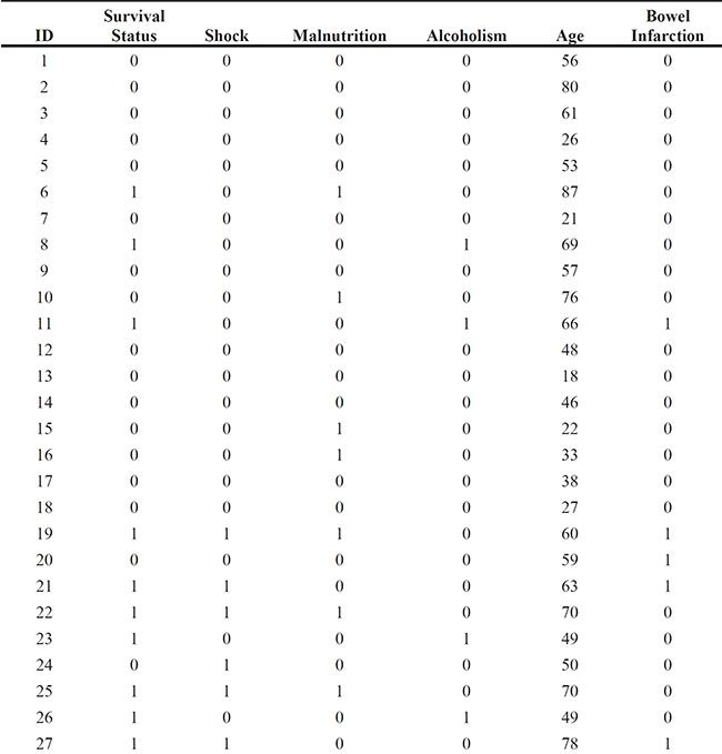

Note that shock, malnutrition, alcoholism, and bowel infarction are binary variables coded as 1 if the symptom was present and 0 if it was absent. Survival status is coded as 1 for death and 0 for alive. Age is given in years.
7.2.1 Intra-Abdominal Sepsis: Using Logistic Regression to Answer the Question of What Predicts Survival after Surgery
The multiple regression model considered in the previous chapter is suitable for investigating how a continuous response variable depends on a set of explanatory variables. But can it be adapted to model a binary response variable? For example, in Table 7.1, a patient’s survival after surgery is such a binary response variable, and we would like to investigate how it is affected by the other variables in the data set. A possible way to proceed is to consider modelling the probability that the binary response takes the value 1 (that is, in our particular example, the probability that a patient dies after surgery for intra-abdominal sepsis). A little thought shows that the multiple regression model cannot help us here. Firstly, the assumption that the response is normally distributed conditional on the explanatory variables is clearly no longer justified. And there is another fundamental problem: the application of the multiple regression model to the probability that the binary response takes the value 1 could lead to fitted values outside the range of 0 to 1, clearly unacceptable for the probability being modelled.
7.2.2 Odds
So, with a binary response variable, we need to consider an alternative approach to multiple regression, and the most common alternative is known as logistic regression. Here the logarithm of the odds of the response variable being 1 (often known as the logit transformation of the probability) is modelled as a linear function of the explanatory variables. Odds were discussed in Chapter 3, where we saw that they are simply the ratio of the probability that the binary variable takes the value 1 to the probability that the variable takes the value 0. Representing the probability of a 1 as p, so that the probability of a 0 is (1-p), then the odds are simply given by p/(1-p). So, for example, when tossing an unbiased die, the odds of getting a 6 are 1/6 divided by 5/6, giving the value 1/5. An experienced gambler would say that the odds of a 6 are 5 to 1 against.
But back to the logistic regression model, which in mathematical terms can be written as:
where x1, x2,....,xq are the q explanatory variables. Now as p varies between 0 and 1, the logit transformation of p varies between minus and plus infinity, thus removing directly one of the problems mentioned above (that is, an estimated probability outside the range [0, 1]). The logistic model can be rewritten in terms of the probability p as:
Full details of the distributional assumptions of the model and how the parameters in the model are estimated are given in Der and Everitt (2013), but essentially a binomial distribution is assumed for the response and then the parameters in the model are estimated by maximum likelihood. Below, however, we shall concentrate on how to obtain estimates of the parameters, β0, β1, β2,....,βq, using SAS University Edition and how to interpret the estimates after we find them.
7.2.3 Applying the Logistic Regression Model with a Single Explanatory Variable
To begin, we shall apply the logistic regression model to the data in Table 7.1 using shock as the single explanatory variable; considering this very simple model should help clarify various aspects of the model before we proceed to consider a more complex model involving all five explanatory variables. But before fitting the logistic model, it will be helpful to look at the cross-classification of survival and shock. This we can find using the following instructions:
1. Open Tasks ▶ Statistics ▶ Table Analysis.
2. Under Data ▶ Data, add sasue.sepsis.
3. Under Data ▶ Roles, add survival to the row variables and shock to the column variables.
4. Click Run.
The edited output just showing the table of interest is given in Output 7.1.
Output 7.1: 2 X 2 Table for Shock and Survival

From this table, we can estimate the probability of death for a patient who has shock as 8/10=0.80 and the corresponding probability for a patient who does not have shock as 10/40=0.25.
Now we can move on and fit the logistic regression model with shock as the only explanatory variable. This model can be written explicitly as:
The model can be fitted using the following instructions:
1. Open Tasks ▶ Statistics ▶ Binary Logistic Regression.
2. Under Data ▶ Data, add sasue.sepsis.
3. Under Data ▶ Roles ▶ Response, add survival and select the Event of interest to be 1.
4. Under Data ▶ Roles ▶ Explanatory Variable ▶ Continuous Variables, add shock.
5. Under Model ▶ Model Effects, select shock and click Add.
6. Click Run.
Output 7.2: Results from Fitting the Logistic Regression Model to the Survival from Surgery Data with a Single Explanatory Variable, Shock


The output of most interest is shown in Output 7.2. Here we find the estimates of the two regression coefficients in the model as and (the ‘hats’ denote sample estimates of the parameters in the model rather than population values). The fitted model is therefore
So for Shock=0 (no shock), this gives
And the corresponding calculation for Shock=1 gives . These two estimates are, of course, equal to those derived previously based on the 2 x 2 contingency table of survival against shock.
Now let us look at another logistic regression model again with a single explanatory variable, the age of the patient; we can do this by making changes to the settings of the previous task:
1. Click the Binary Logistic Regression tab.
2. Under Data ▶ Roles ▶ Explanatory Variables ▶ Continuous Variables, add age and remove shock.
3. Under Model ▶ Model Effects, select age and click Add.
4. Click Run.
The edited output is shown in Output 7.3. The first part of the output simply gives information about the data set being analysed and the technique used for getting the estimate of the regression coefficients in the model. The statement that the probability modelled is Survival=1 means that it is the probability of death which is modelled, as the variable survival takes the value 1 for a patient who dies. Then the estimated regression coefficients are given with their estimated standard errors. Here, of course, it is the regression coefficient for age that is of interest and three tests of the hypothesis that the population regression coefficient takes the value 0 are given. As sample size increases, these different tests lead to the same conclusion--namely, that there is strong evidence that the regression coefficient is not 0. (For a discussion of the details of the three tests, see Collett, 2003.) To help in the interpretation of the fitted model, a confidence interval for the odds ratio is given (see Chapter 3); here, the 95% confidence interval is [1.03, 1.13]. This implies that an extra year of age increases the odds of not surviving surgery for intra-abdominal sepsis between about 3% and 13% over the odds of surviving surgery in this population of patients.
It is helpful to look at a graphic representation of the fitted model, in this case a plot of the estimated probability of dying from surgery against age. We can obtain this plot using the following instructions:
1. Click the Binary Logistic Regression tab.
2. Under Options ▶ Plots ▶ Select Plots to Display, select Default & additional plots.
3. From the resulting list, select Effect plot.
4. Click Run.
The resulting plot appears in Figure 7.1. This plot clearly demonstrates the effect of aging on the probability of dying from surgery.
Output 7.3: Edited Output from Fitting a Logistic Model to the Data in Table 7.1 with Age as the Single Explanatory Variable
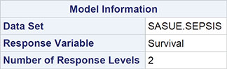


Probability modeled is Survival=1.
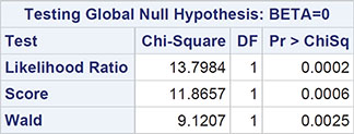


Figure 7.1: Plot of Predicted Probabilities from Logistic Regression Model with Age as the Single Explanatory Variable Fitted to Data in Table 7.1 Against Age

7.2.4 Logistic Regression with All the Explanatory Variables
So finally we can consider a logistic model incorporating all five explanatory variables by amending the previous task as follows:
1. Click the Binary Logistic Regression tab.
2. Under Data ▶ Explanatory Variables ▶ Continuous Variables, add shock, malnutrition, alcoholism, and bowel_infarc.
3. Under Model ▶ Variables, select all the variables and click Add.
4. Click Run.
The edited results are shown in Output 7.4. Examining each of the estimated regression coefficients and their corresponding p-values, we would conclude that age, shock, and alcoholism are the important explanatory variables in the prediction of the probability of dying from surgery for intra-abdominal sepsis because the regression coefficients for these variables are all significantly different from 0; aging, the presence of shock, and alcoholism all increase the probability of dying from surgery. One problem with these results is that the relatively small sample size leads to very wide confidence intervals for the associated odds ratios of shock and alcoholism, so we need to be cautious about interpreting the effects of these explanatory variables on survival from surgery. Nevertheless, it is pretty clear that the news for alcoholic patients who suffer shock is not good; their chance of surviving surgery is considerably less than their non-alcoholic and shock-free fellow patients.
We also need to be careful in interpreting each estimated regression coefficient in Output 7.4 in isolation because the explanatory variables are not independent of one another and the same applies to the estimated regression coefficients, a point raised previously in Chapter 6 when we discussed multiple regression models. Removing one of the variables, for example, and refitting the model would lead to different estimated regression coefficients for the variables remaining in the model than for those given in Output 7.4. For this reason, methods for selecting the best set of explanatory variables have been developed when using logistic regression models that are similar to those used in Chapter 6 for multiple regression models, although the criteria used for judging when variables should be removed or entered into an existing model are different. Details are given in Der and Everitt (2013) and exercise 7.5 invites keen readers to apply these variable selection methods for logistic regression to a data set.
Output 7.4: Parameter Estimates and Standard Errors for the Logistic Regression Model with All Five Explanatory Variables Fitted to the Data in Table 7.1


7.2.5 A Second Example of the Use of Logistic Regression
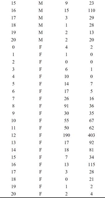
Goldberg (1972) describes a psychiatric screening questionnaire, the General Health Questionnaire (GHQ), designed to identify people who might be suffering from a psychiatric illness. In Table 7.2, some results from applying this instrument are given; here what is of interest is how the probability of being classified as a potential psychiatric case by a psychiatrist is related to an individual’s score on the GHQ and the individual’s gender. Note that the data here have been grouped in terms of the binary variable, caseness, value of yes or no. So, for example, there are four women with a GHQ score of 0 rated as cases and 80 women with a GHQ of 0 rated as non-cases.
Table 7.2: Psychiatric Caseness Data

7.2.6 An Initial Look at the Caseness Data
A good way to begin to understand the data in Table 7.2 is to plot the estimated probability of being a case against the GHQ score, identifying males and females on the plot.
In addition to the four variables shown in Table 7.2, the data set sasue.ghq contains two further variables: total, the sum of cases and noncases, and prcase, the number of cases divided by the total. We use the prcase variable to construct the plot:
1. Open Tasks ▶ Graph ▶ Scatter Plot.
2. Under Data ▶ Data, select sasue.ghq.
3. Under Data ▶ Roles, select score as the x variable,; prcase as the y variable, and sex as the group variable.
4. Click Run.
Figure 7.2: Plot of Estimated Probability of Being a Case Against the GHQ Score for the Data in Table 7.2
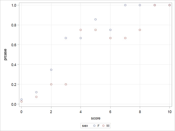
The resulting plot is shown in Figure 7.2. Clearly the estimated probability of being considered a case increases with the increasing GHQ score. For most values of GHQ, women have a higher estimated probability of being considered a case than men, but there is a reversal around a GHQ score of 4. In the next section, we shall fit a logistic model to the caseness data that is suggested by the plot in Figure 7.2.
7.2.7 Modeling the Caseness Data Using Logistic Regression
As suggested by Figure 7.2, we want to fit a model that models the relationship between the probability being considered a case and the GHQ score that allows for both a possible sex difference and a possible change in any sex difference over the range of GHQ scores. Such a model has to have explanatory variables for the GHQ score, for the sex, and for the interaction term score x sex; it is this latter term that allows for the possibility that any sex difference depends on the GHQ score in some way. We can write the required model explicitly as
So for men with sex=1, the model can be rewritten as
And for women with sex=0, we have
The necessary instructions for fitting this model are:
1. Open Tasks ▶ Statistics ▶ Binary Logistic Regression.
2. Under Data ▶ Data, select sasue.ghq.
3. Under Data ▶ Roles ▶ Response, select Response data consists of number of events and trials.
4. Add cases as the number of events.
5. Add total as the number of trials.
6. Under Data ▶ Roles ▶ Explanatory Variables ▶ Classification Variables, add sex and under Parameterization of Effects, select Reference coding.
7. Under Data ▶ Roles ▶ Explanatory Variables ▶ Continuous Variables, add score.
8. Under Model ▶ Model Effects, select both variables and click Full Factorial. This is equivalent to selecting both and then clicking Add and Cross.
9. Under Options ▶ Plots, select Default & additional plots and then select Effect plot.
10. Click Run.
The parameter estimates and their standard errors are shown in Output 7.5 and the plot representing the fitted model is shown in Figure 7.3.
Output 7.5: Parameter Estimates for the Interaction Model Fitted to the Caseness Data

Figure 7.3: Plot of Predicted Probability of Caseness from the Interaction Model Fitted to the Caseness Data

Looking at the parameter estimates in Output 7.5, we see that there is no evidence that the regression coefficients for sex or the interaction of sex and the GHQ score differ from 0. But we should now fit a model that includes both sex and GHQ score, rather than dropping both the interaction of sex with score and sex at the same time, because these two effects are confounded. So now let us fit a logistic regression model with sex and score as the two explanatory variables:
1. Click the Binary Logistic Regression tab. (If it has been closed, repeat steps 1 to 8 above.)
2. Under Model ▶ Model Effects, delete score*sex from the model effects--that is, select it and click the Delete button (![]() ).
).
3. Click Run.
The estimated regression coefficients for this model are shown in Output 7.6 along with the estimated odds ratio estimate for both the GHQ score and sex and the associated 95% confidence intervals. The model fit statistics have been discussed in the previous chapter and are essentially for use in comparing two competing models (see the next chapter for more details). The Wald chi-squared statistic is simply the square of the ratio of the estimated regression coefficient to its estimated standard error and is tested as a chi-square with a single degree of freedom. Both sex and GHQ score are significant at the 5% level. The confidence intervals show that conditional on sex, a one-point increase in the GHQ score leads to between about an 80% and a 160% increase in the odds of being judged a case rather than a non-case. It also shows that for a given GHQ score, there is between about an 8% and a 500% increase in the odds of being judged a case rather than a non-case for women compared to men. The plot representing the fitted model is shown in Figure 7.4.
Output 7.6: Results from Fitting a Logistic Regression Model with GHQ Score and Sex as Explanatory Variables to the Psychiatric Caseness Data
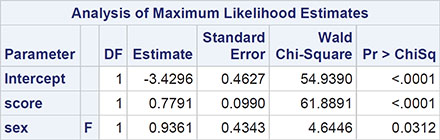

Figure 7.4: Plot of Predicted Probability of Caseness from the Model with Sex and GHQ Score Fitted to the Caseness Data

(A more detailed analysis of the caseness data is given in Der and Everitt, 2013.)
7.3 Logistic Regression for 1:1 Matched Studies
A frequently used type of study design, particularly in medical investigations, is known as the matched case-control design, in which each person having a particular condition of interest is matched to one or more people without the condition on variables such as age, gender, ethnic group, and so on. A design with m controls per case is known as a 1:m matched study. In many cases, m will be 1, and it is the 1-1 matched study that we shall concentrate on here.
The example we shall consider involves the birth weight of babies. The data arise from looking first at 59 babies who were low weight, defined as weighing less than 2,500 g. The matched data were obtained by randomly selecting for each woman who gave birth to a low birth weight baby, a mother of the same age who did not give birth to a low birth weight baby. Three of the low birth weight mothers were too young to find a match, so the data consist of 56 matched case-control pairs. The complete data are given in Hosmer and Lemeshow (2000), with data for the first five matched pairs given here in Table 7.3. Variables selected for investigation were prior pre-term delivery (ptd, 1=yes, 0=no), smoking status of the mother during pregnancy (smoke, 1=yes, 0=no), history of hypertension (ht, 1=yes, 0=no), presence of uterine irritability (ui, 1=yes, 0=no), and the weight of the mother at the last menstrual period (lwt, pounds).
Table 7.3: Part of the Data from the Matched Case-Control Study of Babies by Birth Weight

LOW |
Low Birth Weight |
AGE |
Age of Mother |
LWT |
Weight of Mother at Last Menstrual Period |
SMOKE |
Smoking Status During Pregnancy |
PTD |
History of Premature Labor |
HT |
History of Hypertension |
UI |
Presence of Uterine Irritability |
For a single explanatory variable x, for example, the smoking status during pregnancy in the birth weight data, the form of the logistic model used for matched data involves the probability, φ, that in matched pair i, for a given value of smoking status during pregnancy (yes, or no), the member of the pair is a case. Specifically the model is
logit(φ)=αi+βx
The odds that a subject who smokes during pregnancy (x = 1) is a low birth weight case equals exp(β) times the odds that a subject who does not smoke (x = 0) is a low birth weight case. The αi terms model the shared values of the ith pair on the matching variables.
The model generalizes to the situation where there are q explanatory variables as
logit(φ)=αi+β1+x1+...αqxq
Typically, one xi is an explanatory variable of real interest, such as past exposure to smoking in the example above, with the others being used as a form of statistical control in addition to the variables already controlled by virtue of using them to form matched pairs. The problem with the model above is that the number of parameters increases at the same rate as the sample size, with the consequence that maximum likelihood estimation is no longer viable. We can overcome this problem if we regard the parameters αi as of little interest and so are willing to forgo their estimation. If we do, we can then create a conditional likelihood function that will yield maximum conditional likelihood estimators of the coefficients, β1...βq, that are consistent and asymptotically normally distributed. Essentially, the conditioning avoids the estimation of the parameters accounting for the matching. The mathematics behind this are described in Collett (2003), but the parameters for the explanatory variables in the model have the same log odds ratio interpretation familiar from the standard logistic model The result is that we can conduct the regression analyses exactly as before. However, the variables used in matching are controlled for automatically and so not used directly in modeling. Here we concentrate on how to fit such a model to the low birth weight data and how to interpret the resulting parameter estimates. We begin with a simple model that only considers the smoking status during pregnancy:
1. Open Tasks ▶ Statistics ▶ Binary Logistic Regression.
2. Under Data ▶ Data, add sasue.lbwpairs.
3. Under Data ▶ Roles ▶ Response, add low and select the Event of interest to be 1.
4. Under Data ▶ Roles ▶ Explanatory Variable ▶ Continuous Variables, add smoke.
5. Under Model ▶ Model Effects, select smoke and click Add.
We now need to edit the code produced so far.
6. In the code pane, click Edit.
A program pane opens that contains the following code:
proc logistic data=SASUE.LBWPAIRS plots;
model low(event='1')=Smoke / link=logit technique=fisher;
run;
7. Before the RUN statement, add
strata pair;
Take care to include the semicolon at the end.
8. Click Run.
The results are shown in Output 7.7. The 95% confidence interval for the odds ratio is [1.224, 6.177]. This implies that in a matched pair of women, the odds that the mother of a low birthweight baby smoked during pregnancy, are estimated to be between about 1.2 and 6.2 times the odds that the control mother, one not having a low birthweight baby, has smoked during pregnancy.
Output 7.7: Parameter Estimates for the Logistic Regression Model Applied to the Matched Low Birth Weight Data Using Smoking During Pregnancy as the Single Explanatory Variable


We now fit the model with all the explanatory variables by further edits to the code produced above:
1. Select the program window containing the edited code.
2. Type in the names of the other explanatory variables (lwt, ptd, ht, and ui) on the MODEL statement so that the resulting code now is
proc logistic data=SASUE.LBWPAIRS;
model low(event='1')=Smoke lwt ptd ht ui / link=logit
technique=fisher;
strata pair;
run;
3. Click Run.
The results are shown in Output 7.8.
Output 7.8: Results from Fitting Logistic Regression to the Matched Birth Weight Data Using All Variables


Probability modeled is low=1.

Newton-Raphson Ridge Optimization
Without Parameter Scaling
Convergence criterion (GCONV=1E-8) satisfied.


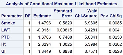


The estimated odds ratios in Output 7.8 indicate that smoking during pregnancy, prior preterm deliveries, and the presence of hypertension are important risk factors for delivering a low birth weight baby. The confidence intervals associated with the dichotomous variables are very wide, which largely results from the sparsity of discordant pairs. Hosmer and Lemeshow (2005) point out that the gain in precision obtained from matching and using conditional logistic regression may be offset by a loss owing to there being only a few discordant pairs for dichotomous covariates.
7.4 Summary
Logistic regression models are very widely used in many disciplines but particularly in medical studies. In this chapter, we have tried to describe how to interpret the estimated parameters from such models. As with multiple regression models, a complete analysis of a data set using logistic regression should involve diagnostic plots for assessing the assumptions made by these models. Such diagnostic plots are provided by SAS University Edition, but we have not discussed them here because they are technically quite complicated and, in our experience, they are not always helpful in shedding light on whether a model is suitable for a particular data set. Full details of diagnostic plots for logistic regression models are, however, given in Collett (2003) for readers who are anxious that they may be missing something of importance.
7.5 Exercises
Exercise 7.1: Plasma Data
The data set plasma was collected to examine the extent to which erythrocyte sedimentation rate (ESR), the rate at which red blood cells (erythocytes) settle out of suspension in blood plasma, is related to two plasma proteins, fibrinogen and ![]() -globulin, both measured in gm/l. The ESR for a healthy individual should be less than 20mm/h and because the absolute value of ESR is relatively unimportant, the response variable used here denotes whether this is the case. A response of 0 signifies a healthy individual (ESR<20), while a response of unity refers to an unhealthy individual (ESR≥20). The aim of the analysis for these data is to determine the strength of any relationship between the ESR level and the levels of the two plasmas. Investigate the relationship by fitting a logistic model for the probability of an unhealthy individual with fibrinogen and gamma as the two explanatory variables. What are your conclusions?
-globulin, both measured in gm/l. The ESR for a healthy individual should be less than 20mm/h and because the absolute value of ESR is relatively unimportant, the response variable used here denotes whether this is the case. A response of 0 signifies a healthy individual (ESR<20), while a response of unity refers to an unhealthy individual (ESR≥20). The aim of the analysis for these data is to determine the strength of any relationship between the ESR level and the levels of the two plasmas. Investigate the relationship by fitting a logistic model for the probability of an unhealthy individual with fibrinogen and gamma as the two explanatory variables. What are your conclusions?

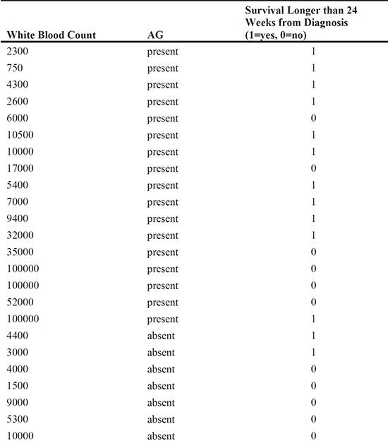
Exercise 7.2: Leukaemia Data
The data in leukaemia2 report whether patients with leukaemia lived for at least 24 weeks after diagnosis, along with the values of two explanatory variables, the white blood count and the presence or absence of a morphological characteristic of the white blood cells (AG). The data are from Venables and Ripley (1994). Fit a logistic regression model to the data to determine whether the explanatory variables are predictive of survival longer than 24 weeks. (You may need to consider an interaction term.)

Exercise 7.3: Low Birth Weight Data
The data in lowbwgt comprise part of the data set given in Hosmer and Lemeshow (1989), collected during a study to identify risk factors associated with giving birth to a low birth weight baby, defined as weighing less than 2,500 grams. The risk factors considered were the age of the mother, the weight of the mother at her last menstrual period, the race of the mother, and the number of physician visits during the first trimester of the pregnancy. Fit a logistic regression model for the probability of a low birth weight infant using age, lwt, race (coded in terms of two dummy variables), and ftv as explanatory variables. What conclusions do you draw from the fitted model?

LOW : |
0 = weight of baby > 2,500 g |
|
1 = weight of baby <= 2,500 g |
AGE : |
Age of mother in years |
LWT : |
Weight of mother at last menstrual period |
RACE : |
1 = white, 2 = black, 3 = other |
FTV : |
Number of physician visits in the first trimester |
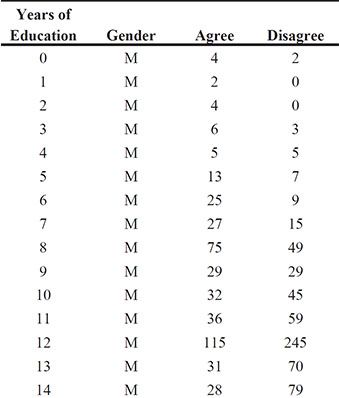
Exercise 7.4: Role Data
In a survey carried out in 1974 and 1975, each respondent was asked if he or she agreed or disagreed with the following statement: Women should take care of running their homes and leave running the country to men. The responses are summarized in the role data set (from Haberman, 1973) and are also given in Collett (2003). The questions of interest here are whether the responses of men and women differ and how years of education affect the response given. Fit appropriate logistic regression models to answer these questions.
Exercise 7.5: Backward Elimination
Investigate the use of backward elimination in the context of logistic regression modelling to try to find a more parsimonious model for the low birth weight data in Table 7.14.
Exercise 7.6: Acute Herniated Lumber Disc Data
Kelsey and Hardy (1975) describe a study designed to investigate whether driving a car is a risk factor for lower back pain resulting from acute herniated lumber invertebral discs (AHLID). A case-control study was used with cases selected from people who had recently had X-rays taken of the lower back and who had been diagnosed as having AHLID. The controls were taken from patients admitted to the same hospital as a case with a condition unrelated to the spine. Further matching was made on age and sex and a total of 217 matched pairs were recruited, consisting of 89 female pairs and 128 male pairs. The complete data are available in the ahlid data set. Only a part is shown here:

Fit a conditional logistic regression model to the data to determine whether driving and area of residence are risk factors for AHLID.