
Financial Risk Management Metrics
Introduction
As stressed in Chapter 3, one of the essential elements of a financial risk management framework is the measurement of the risks of an organization; measurement of both the existing risks as well as the potential risks going forward. The measurement of risks is obviously one of the most quantitative aspects of risk management. As such, it has the reputation of being the one task of risk management that is best left to the specialists; the quantitative analysts, more commonly called the “quants.” We do not agree with that sentiment. Although the details of the calculations are beyond the scope and intentions of this book, the essentials of financial risk metrics are easily learned, and need to be learned by everyone connected with financial risk management.
In this chapter, we are going to introduce the major financial risk management metrics and explain both how they are used and misused. We are not going to go into the details of the calculations. Many of the calculations are already embedded in risk management software, and even generic spreadsheet programs like Microsoft Excel can calculate most of them almost automatically. Our aim in this chapter is to familiarize the generalist so they can conduct a useful conversation around risk—which by itself necessitates a working knowledge of risk metrics.
Before looking at specific metrics, it is important here to mention a theme that arises at several places in this book, and in this chapter. This theme is that risk management, and financial risk management in particular, is as much of an art as it is a science. Financial risk management concerns itself with a lot of variables that we can easily fool ourselves into thinking that we can measure with unlimited accuracy and precision. For instance, we talk about interest rate changes, the volatility of stock prices, and the range of gold prices, and so on. The reality is that just because we can put a number on something does not mean that we necessarily understand that variable, or that the variable will remain constant, or perhaps most importantly, that the variable we took the time to measure is even an important variable. Often, we get so excited when we can measure something that we forget to ask if it is worth measuring.
In our own educations, we were told to never start a calculation until you have an idea of what the answer should be. This is very valuable advice for risk managers. The risk calculations can become very complicated. Thus, there is the chance that we become enamored with the calculation while forgetting what the objective was. Not using intuition to develop an idea of what the answer should be before starting a formal measurement and calculation also sets the stage for a higher probability of mistakes in the calculation. If the calculation answer or measurement is far from the answer developed through intuition, then we have reason to check both our calculated answer as well as our intuition. In either case, we will find a mistake in our measurement/calculation or our intuition. At best, we correct a calculation mistake, or we develop our intuition a bit more; both good outcomes. If we have no intuitive idea of what the result of a measurement or calculation should be, then we will have no basis for judging if the answer is valid or not.
In our real-life experience, we have been in numerous situations where an experienced manager has given an intuitive answer that differed greatly from the calculated answer produced by a highly trained “quant.” Almost always, the experienced manager was correct and the quant had either a mistake in calculation or a mistake in understanding the workings of the market. We believe that there is a valuable lesson in what we have observed in our own experience.
Historical Relationships
The best place to start with an assessment of risk is by measuring how risk variables and relationships performed in the past. While this is a good starting place, it is just that, a starting place. Risk is dynamic and risk relationships change. Later in this chapter, we will talk about model risk, which in part is caused by assuming that historical relationships will hold going forward. Model risk was one of the key causes of the 2008 financial crisis; quantitative risk analysts assumed that historical default relationships would continue to hold. Those default relationships did not stay constant and valuations that were considered impossible not only became possible but were smashed in reality. The point that must not be forgotten is that economic relationships are notoriously unstable.
The place to start with risk metrics is with correlations. Correlation is simply how closely two variables tend to move together. Variables that tend to move together upwards or downwards are positively correlated, while variables that tend to move in opposite directions are negatively correlated. For instance, stock prices, particularly stocks of companies in the same industry, tend to move together. Bond prices are negatively correlated with interest rates; as interest rates increase, bond prices tend to fall. Correlation values range from plus one to negative one. Two things that are perfectly correlated, so that they move in perfect lockstep, have a correlation of plus one. Likewise, variables that move perfectly opposite to each other so that when one variable is increasing the other is decreasing will have a correlation of negative one. Variables whose changes in value have no relation to each other have a correlation of zero. With real economic variables, there are no two variables that will have a perfect correlation of either a plus one or a negative one.
Correlation is important in risk management for several reasons. Correlations give a measure of sensitivity. For instance, one key risk variable is the sensitivity of sales to an economic variable such as interest rates. The elasticity of sales to interest rates (or other variables such as GDP growth) is a key part of financial risk analysis and a basic use of correlation analysis. Furthermore, costs of goods sold may be correlated to commodity prices or rates of wage inflation. Knowledge of these correlations or sensitivities and the size of these sensitivities help to both prioritize risks from most to least important and to begin the formulation of a risk management plan.
A second reason correlation is important as it helps to decide what to use as hedging instruments. If a firm is trying to eliminate a financial risk by hedging, then they want the hedging instrument they are using to have a high correlation with the variable they are concerned about. For instance, airlines need to hedge jet fuel costs (see case study on Southwest Airlines in Chapter 2). To hedge jet fuel, airlines will often enter into forward or option contracts on oil, since oil prices are highly correlated with jet fuel prices. To the extent that the correlation between the variable the firm is trying to hedge does not have a perfect correlation with the hedge instrument, there is said to be basis risk. The bigger the basis risk, the greater the chance that the hedge will not perform as desired. (Basis risk will be covered in more detail in Chapter 9 on Commodity Risk.)
Since interest rates are such an important financial risk variable, a special type of correlation is calculated called a DV01. To determine interest rate sensitivity, firms need to calculate the change in the value of their debt portfolio. This is usually done by calculating the change in value for a one basis point change in the interest rate, or the yield curve. This change in value for a theoretical one basis point change in interest rates is commonly known as “Dollar Value of a Basis Point,” also known as “DV01.” It is also sometimes called the “Present Value of a Basis Point,” or “PV01.” Many firms will also calculate a DV01 for a one basis point change in an exchange rate as a measure of their currency risk.
Calculation of correlations, or even the DV01, gives a firm a sense of how sensitive various parts of their operations are to changes in different economic variables. These correlations are a starting place for prioritizing the portfolio of risks that the firm faces. There are a couple of caveats to remember when using correlations. To begin, correlations may only hold over a small range or normal variable measures. For instance, at the time of this writing, interest rates have been abnormally low over the last decade since the 2008 financial crisis. Many traditional correlations have significantly changed and current calculations of correlation are unlikely to hold if interest rates increase to more traditional levels. Correlations are also a poor guide when extreme changes in conditions are experienced. This is especially true for DV01 calculations which are designed to measure the variable relationship for a small change in the economic variable (that is for one basis point changes). Finally, correlations tend to change during a crisis. An old adage is that all economic correlations go to one when a crisis hits, or in other words, everything tends to go down in lockstep when a crisis occurs.
Correlations are good for measuring how a variable such as sales is related to changes in one economic variable. Regression analysis is used when there might be more than one variable affecting the variables and when a measure is needed of the size of the effect. Regression analysis is simply a technique to relate the sensitivity of a variable, such as sales, to a number of different factors, such as interest rates, GDP growth, employment levels, and average earned income, simultaneously. Instead of calculating the correlations individually, a regression equation creates a formula relating the various factors to the variable in question. If one has a prediction for each of the factors in the regression equation, for instance, if one has a projection for interest rates, GDP growth, employment levels, and earned income, then one can use the results of a regression analysis to project an estimate for what sales might be.
One special regression equation for companies that have publicly traded equity is to regress the return of the company’s stock returns versus interest rates and the return of the market index. The coefficient of regression for the return of the stock versus the return of the market index gives an indication of the market’s perception of the overall riskiness of a company relative to other publicly traded stocks. This value is called beta. A stock with average riskiness will have a beta close to one, while a riskier-than-average stock will have a beta greater than one. Likewise, a lower-than-average-risk stock will have a beta less than one. Although there are several valid criticisms of the beta measure, the reality is that it is used by a significant number of analysts and investors to gauge the overall riskiness of a firm.
The riskiness of a variable is frequently measured by its standard deviation. Standard deviation is a measure of how much a variable moves around its historical average. The bigger the variation, the more risky the variable is. Standard deviation is generally based in the theory of the normal distribution; the normal bell-shaped curve. Figure 4.1 shows two variables that are normally distributed. While both of our hypothetical variables have the same expected value, the solid curve demonstrates more dispersion, or has the fatter distribution. Thus, the solid curve has the higher standard deviation and would be considered the higher risk variable.

Figure 4.1 Table showing distribution of two hypothetical economic variables
The variable represented by the solid line has the higher standard deviation.
Standard deviation is a useful variable if the variable in question is normally distributed, that is, it has the frequency of outcomes that approximate the bell-shaped curve represented in Figure 4.1. The normal distribution is symmetric in that results that are above average occur with the same frequency as the results that are below average. However, standard deviation is a poor measure of risk if the distribution is skewed, which is the case as shown in Figure 4.2. Figure 4.2 shows the frequencies of outcomes of a variable with positive skew. A variable with negative skew would have the long tail going toward negative values.

Figure 4.2 Variable with positive skew
Examining the skew of a distribution is important as skew indicates whether there is more upside or downside potential. Standard deviation assumes that the distribution is symmetric, while skew gives an indication of a bias to the upside or the downside.
Another measure of risk that explicitly takes into account the upside-versus-downside variation is a measure known as semi-standard deviation. Instead of just calculating a measure of the deviations from the mean, like standard deviation does, semi-standard deviation separately calculates the level of the upside deviations separate from the level deviations on the downside. Semi-standard deviation thus allows a ratio of the upside risk to the downside risk to be calculated.
Standard deviation and the more advanced semi-standard deviation are powerful metrics that provide a picture to the variability of various economic variables. They are thus another component to rank and prioritize risks.
Monte Carlo Simulation
Once the various sensitivities between the firm’s variables, and the correlations and regression factors to external financial or economic variables have been calculated, along with a measurement of how much each of the economic variables has varied in the past, then a series of forecasting techniques can be used to project how the firm might behave going forward.
One method to do so is scenario analysis. A scenario analysis is frequently done as part of the conventional economic plan. However, scenario analysis is also very useful for planning risk management strategies, and for assessing the potential outcomes of implementing such risk management strategies. The value in scenario analysis is not that any of the developed scenarios will ever occur—the probability of that happening even approximately is extremely low—but in developing intuition of how the variables affecting the firm are interrelated. In the classic reference for scenario analysis written by Peter Schwartz, he claims that good scenario analysis should be like a story1. For risk management purposes, scenario analysis should go beyond and be like a very creative story, as risk management needs to be able to handle the extreme unexpected outcomes.
Many corporations limit themselves to developing scenarios for an expected case, best case, and a worse case. However, the more scenarios that can be developed, the better. Using the correlations and regression models, combined with the standard deviations of the underlying economic variables, one can use a technique called Monte Carlo Simulation to develop thousands of potential outcomes. To develop a Monte Carlo Simulation, a company will build a model for the major outcomes of the firm—for instance, the income statement. For each line of the income statement, it will build in an equation of how that variable is correlated to underlying economic variables. For instance, sales might be correlated to interest rates and GDP growth, while expenses might be correlated to the cost of an input commodity. A computer model can then calculate the sales and costs, and the resulting net income by selecting thousands of possible values for the underlying economic variables using the historical frequency curves for those underlying variables. Thus, instead of creating one or two possible future scenarios, the computer generates thousands of different scenarios or simulations that are consistent with the observed distributions of the underlying variables. The output from a Monte Carlo Simulation is a frequency curve (or table) for the underlying sales, expenses, and net income. Although it sounds very complicated, in reality it is very easy to do and several user-friendly computer packages exist to make the process relatively quick and easy to do.
Monte Carlo Simulation is a very powerful technique for analyzing risk. It shows the distribution of possible outcomes going forward, based on how the underlying variables have performed in the past. Once a Monte Carlo Simulation is set up, it is relatively easy to run different simulations and examine outcomes from utilizing different risk management strategies. This provides a powerful picture of how the future will look, given different risk management strategies.
The fact that the output from a Monte Carlo Simulation is a distribution of possible values is a distinct advantage for the technique. While some managers may prefer to receive a single number for forecasting the future, the reality is that we cannot forecast an uncertain future in such a precise manner. A Monte Carlo Simulation explicitly recognizes this and thus forecasts a distribution of potential outcomes, which is closer to the reality of what we can at best predict. While Monte Carlo does not give a unique answer, it does give a realistic range of answers—that is, a realistic range or distribution of outcomes. It forces managers to think in terms of distributions instead of single numbers, which in our belief is a better way to do the analysis.
There is one main drawback to using a Monte Carlo Simulation. A Monte Carlo Simulation is only as good as the model used to build it, and the distributions used for the underlying economic variables. If a company does not have a good understanding of how its variables of importance such as sales or costs are related to economic variables, then the results of the Monte Carlo Simulation will not be accurate. Likewise, if the relationships change, or if the distribution of the underlying variables change, then the results may be misleading. However, it is also true that if a company cannot model how their operational results are related to economic variables, then any risk management calculation, and any risk management strategy will likely be suboptimal at best. Understanding how the operations of the firm are affected by external factors is an issue of understanding the business, not necessarily a risk issue.
Value at Risk (VAR)
Value at Risk, commonly known as VAR, has become a popular technique that combines many of the principles of Monte Carlo Simulation but distills the results into a single number. VAR was originally developed for financial institutions as a method to give them an estimate of their potential daily losses. Variations of VAR for nonfinancial corporations include Cash Flow at Risk and Earnings at Risk.
With a typical VAR calculation, a Monte Carlo is performed on the forecasted value of the firm (or the forecasted value of the cash flows, or the forecasted value of the expected earnings) and the graph for the distribution of the value if presented. The next step of a VAR calculation is to determine a confidence interval. For financial institutions, this is generally one percent or sometimes a tenth of a percent. For a nonfinancial corporation, a five-percent or a ten-percent confidence level would also be appropriate. For this given confidence level, the value at which there is the probability that the same percentage of forecasted results can then be read off of the distribution graph. This value becomes the VAR. Figure 4.3 illustrates a sample where the confidence level has been chosen to be one percent. In other words, the vertical line is drawn so that one percent of all simulated values of the variable being measured lie to the left of the line. That value is the VAR.
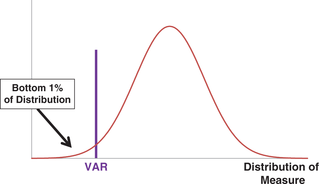
Figure 4.3 Value at risk chart
The VAR calculation is generally done for a given period of time. In other words, the simulation can be done for a day, a quarter, or a year looking forward. Financial institutions usually calculate the VAR for a 10-day period, in part for regulatory reasons. For a nonfinancial corporation, it probably makes more sense to calculate the VAR on a quarterly or yearly basis. Thus, the VAR number is a value of expected downside loss for a given period of time with a given confidence level.
Value at Risk and likewise, Cash Flow at Risk and Earnings at Risk have become popular methods to characterize the riskiness of the firm into a single number. It is a very practical way to examine the usefulness of a proposed risk management strategy as well. The VAR can be calculated assuming no risk management, and again with a variety of different risk management strategies in place. It is one method for calculating the value of risk management by looking at the change in VAR when a risk management strategy is factored into the analysis.
There are a couple of caveats to remember though when using VAR. Firstly, and as with Monte Carlo Simulation, it is a black-box technique in that it is not always possible to back out what the key risk variables are. Secondly, and again in common with the more general Monte Carlo Simulation, it is only as good as the model used to build it. If the managers who build the VAR model do not fully understand and correctly incorporate the economic variables affecting the value of the firm, then the model will give misleading results.
There is also a unique downside to having a single number to characterize the losses that may occur. The VAR measure tells you how much you can expect to lose with a given confidence interval. It is important to understand that it does not tell you how much the loss could be, or what the maximum loss is. Examining Figure 4.2, one needs to realize that there are negative numbers far to the left of the VAR number which represent larger possible loss levels for the firm.
Another unique issue with VAR is that it focuses solely on risk on the downside. Recalling that risk is both the potential for upside gains as well as downside losses, it becomes apparent that VAR is a single-focused measure. For this reason, we prefer to look at the entire results of the Monte Carlo Simulation analysis which shows the entire distribution of upside and downside possibilities. True, the Monte Carlo Simulation does not give you a neat answer as a single number. However, the effort required to examine the entire distribution of results we believe is well worth it.
Dangers of Risk Metrics
Risk metrics are very useful, necessary, and helpful tools for financial risk management. However, financial risk metrics need to be handled with caution as there are some subtle but important inaccuracies and false conclusions that one can make.
To begin this section on the dangers of risk management, consider the reality of what is known as leptokurtosis. There is often an important difference between the theoretical values calculated by the risk quantitative analysts and the realized values that occur in real life. Much of the mathematics used by risk quants is based on the normal distribution. The normal distribution is the bell-shaped distribution that you likely remember from grade school. The normal distribution describes the frequency of various events happening. For many things in real life, it does an excellent job of doing so. Events as diverse as the distribution of heights of a group of people, the distribution of test scores, the distribution of household incomes for a given district, and so on. Given the parameters of the normal distribution, mathematicians can calculate with a high degree of accuracy the number of expected outcomes within a given range.
The normal distribution is also used to calculate the distribution of financial variables and for the most part it works very well. However, it is not perfect. Financial variables are not exactly distributed according to the normal distribution. Most financial variables exhibit what is known as a leptokurtic distribution. In essence, it means that extreme events are more likely to happen in reality than they are as calculated from the normal distribution. Leptokurtosis is also known as “fat-tails,” because the extreme tails of the distribution are fatter than theory says they should be. Table 4.1 illustrates using stock returns from the exchange traded fund SPY (also known as Spyders) which tracks the level of the S&P500 Stock Index.
Table 4.1 Daily returns and actual and theoretical frequencies for the exchange traded fund SPY
| Return bucket | Actual frequency | Theoretical frequency |
| −0.104 | 1 | 0 |
| −0.092 | 1 | 0 |
| −0.080 | 1 | 0 |
| −0.068 | 3 | 0 |
| −0.056 | 5 | 0 |
| −0.044 | 15 | 1 |
| −0.032 | 34 | 21 |
| −0.020 | 175 | 228 |
| −0.008 | 682 | 1,013 |
| 0.004 | 2,461 | 1,855 |
| 0.016 | 1,328 | 1,409 |
| 0.028 | 234 | 443 |
| 0.040 | 62 | 57 |
| 0.052 | 17 | 3 |
| 0.064 | 8 | 0 |
| 0.076 | 2 | 0 |
| 0.088 | 0 | 0 |
| 0.100 | 0 | 0 |
| 0.112 | 1 | 0 |
| 0.124 | 0 | 0 |
| 0.136 | 1 | 0 |
Data for the 20-year period of January 2, 1998–December 29, 2017.
The daily returns for the 20-year period extending from January 2, 1998 to December 29, 2017 were calculated. The first column of Table 4.1 shows the range of “buckets” for returns, while the second column shows the number of days that the actual return did fall into that bucket. The third column shows the theoretical number of returns one should expect given the assumption that stock returns are normally distributed.2 For the lowest bucket of returns, which represents daily returns below a negative 0.104, we see that there was one day where that occurred in reality, while the theoretical expected number of days that it should have occurred was zero. Likewise, for the largest bucket of returns, those days with a return between 0.124 and 0.136, we see that there was one actual day with a return this large, while the expected number of days from the theoretical calculation is again zero. In fact, the actual number of days with a return below a negative 0.044 is 26 days, while the theoretical number of expected days with a return that negative is only one. Likewise, the number of days with a daily return above 0.052 is 29, while the theoretically expected number of days is only three.
Leptokurtosis is the reason why it seems we have a once-in-a-hundred-year move in the market every few years. It is reasonable to ask why risk quants do not use the leptokurtosis distribution in their analysis. The short answer is that there does not exist a mathematical equation to accurately describe leptokurtosis, although it is not from a lack of trying to develop one. For the vast majority of time, the normal distribution works quite well. Additionally, the normal distribution is well known and relatively easy to do calculations with. In fact, the calculations for the above table using the normal distribution were automatically compiled in Excel. The problem is, when you most need an accurate calculation, that is when extreme events are occurring in the financial markets, then that is when the theoretical calculations will be the most inaccurate and misleading. This was the case for the hedge fund Long Term Capital Management (see the case study at the end of the chapter), and this was the case during the lead up to the 2008 financial crisis.
Related to, but not quite equivalent, is the case of Black Swans. A Black Swan is a highly unlikely, but a highly significant event with far-reaching implications. Winning a lottery would be a Black Swan. The events of September 11, 2001 were a rather unfortunate Black Swan. Black Swans are often associated with “fat-tails,” but they should be considered to be different in nature. Whether it is Black Swans, or fat-tails, the implication is the same. One needs to be aware of the assumptions underlying the theoretical calculations of risk events.
Before concluding this chapter, there is one more aspect of risk metrics that is not usually considered, but which is critical for proper risk management. Virtually all of the measures mentioned depend on concepts derived from the mathematics of statistics and probability. These mathematical laws depend on having a large number of observations. This leads to what is called the frequency bias, which has subtle but profound implications for risk management.
To understand the frequency bias, consider the flipping of a coin. Assuming it is a fair coin, you know that it will land heads up fifty percent of the time and heads down fifty percent of the time. Thus, if you were to flip the coin one thousand times, you could be relatively confident that it will land heads up approximately five hundred times. If someone was to make a bet with you, whereby they pay you $1,050 every time the coin landed heads and you had to pay them $1,000 every time it landed up heads, you would quickly calculate that your expected value from each flip was $25. If the net payout was to be made after 1,000 flips of the coin, then you would gladly take this bet as your expected value would be $25,000. However, what if we were lazy and only wanted to flip the coin once. If it came up heads, then you would win $1,050,000. However, if the coin flip produced a tail, then you would lose $1,000,000. Now you would likely think very different about how attractive the bet is, even though statistically they are the same. This example illustrates the frequency bias. We calculate outcomes as if we have an opportunity to do them over and over again many times. However, in real life, we generally only have one or two flips of the coin when it comes to a given business decision. Risk managers ignore this fact at their peril.
Long Term Capital Management
Long Term Capital Management (LTCM) was a hedge fund that was begun by a group of very seasoned investment professionals and two Nobel Prize winning financial specialists. The Nobel Prize winners were Myron Scholes and Robert Merton. Drs. Scholes and Merton, along with their colleague Fischer Black (who had previously passed away) created the famous Black-Scholes-Merton model for pricing financial options and which underlies many of the principles of financial risk management calculations.
The objective of LTCM was to use financial risk management principles for taking investment risk. The partners of the fund assumed that they would be able to take huge levels of risk, and employ very high levels of leverage to earn outsized returns. They would be able to take huge risks because they would hedge those risks with their Nobel Prize winning risk management models.
For the first couple of years of the fund, the strategy worked perfectly. The fund achieved very high level of returns and it seemed as if risk management was a license to print money. However, things started to unravel just a few years into the life of the firm and ultimately the firm went bankrupt and needed to be bailed out in a rescue operation that was coordinated by the U.S. Federal Reserve.
The example of LTCM shows that model risk and the assumptions of risk management will not always hold; regardless of how sophisticated the analysis. LTCM had a small army of highly trained quants. They had the best of analytical equipment. Ultimately it all failed for LTCM.
There are many lessons to be learned from LTCM. The main one is that models are never equivalent to real-world outcomes, and an undue reliance on models has a high probability of leading to ruin.3
Understanding risk metrics is a key skill for everyone involved with risk management. It is not necessarily the calculations that matter—most risk metrics are now done automatically by the data management system in any case. What matters is understanding what the numbers are saying and ensuring that a proper interpretation is being made.
Risk metrics are a powerful and necessary tool for effective financial risk management. However, risk metrics have to be treated with caution. Risk metrics are only as good as the models are to develop them, and only if the mathematical assumptions such as normally distributed variables hold.
Intuition should always be used in conjunction with risk metrics. Remember, financial risk management is as much of an art as it is a science.
________________
1P. Schwartz. 1996. The Art of the Long View: Planning for the Future in an Uncertain World (New York, NY: Currency Doubleday).
2Technically the calculations were done using the assumption of log-normal distributions. The difference between the log-normal distribution and the normal distribution need not bother us here, and the conclusion is the same regardless of which of the two distributional assumptions are made.
3For those interested in learning more about Long Term Capital Management, an excellent rendering and analysis of the situation are given in the book by R. Lowenstein. 2000. When Genius Failed: The Rise and Fall of Long Term Capital Management (New York, NY: Random House).