CHAPTER 7

Alternative Approaches to Valuation

This chapter deals with alternative approaches to company valuation for merger and acquisition (M&A). Naturally, accurate assessment of the value of the target firm in determining the fair price investors should pay for the entity in a competitive market is critically important for the financial success of the acquisition. However, even though determination of a fair price is the necessary condition for success, it is by no means a sufficient condition for the eventual success of the combination because a fair price cannot guarantee smooth, successful postmerger integration of the entities.

Several methods for company valuation exist.¹ In this chapter, we examine three approaches that are listed below:

We note that there are no analytical differences between the spreadsheet approach and the formula approach. They both use discounted cash flow (DCF) analysis and give the same numerical results. The difference is that while the spreadsheet approach presents financial statements over several years, the formula approach expresses the same data compactly in a formula. The spreadsheet approach is more intuitive than the formula approach. We discuss these approaches by using examples next.

Comparable Companies Approach in Company Valuation

This approach uses certain market-based transactions such as market stock price or sales, market stock price or book stock price, and market stock price or net income of comparable companies as a basis for determination of the value of a target company. In the calculation of these ratios, the market price of common stocks refers to the price of common stock of the target company after the conclusion of the merger negotiation.

To find comparable companies, one should consider several variables including:

Let us suppose that we found three companies X, Y, and Z that are comparable to the target company A. The data equity value–sales and price–earnings ratios for the comparable companies and their averages are presented in Table 7.1.

We multiply the average ratios by the actual data of the target company A to calculate its current market price. The recent data of the target company A are those that appear in the first column of Table 7.2. We show the results in the third column of Table 7.2.

According to the adjusted equity value, the investors should pay no more than $111 million for the target.

Note that the ratios in Table 7.1 should be close in value and have minimal variance. Otherwise, the companies are not comparable.

Table 7.1 Comparable companies ratios

Ratio	Firm X	Firm Y	Firm Z	Average
Equity (market)/sales	1.3	1.1	0.9	1.1
Equity (book)/sales	1.1	1.2	1.3	1.2
Equity (market)/net income = P/e	20	15	25	20

Comparable Transactions Method

This method uses the value of some recent comparable M&A transactions in the valuation of the target company. To illustrate how the method works, we use data from Table 7.1. We assume companies X, Y, and Z were involved in the same type of merger transactions as company A plans to conduct.

Since the postannouncement equity price of a typical targeted company is 30 to 40 percent above the company’s equity price before the announcement of the takeover, one should adjust the values in Table 7.1 to reflect the price differential. We assume all ratios in Table 7.1 have increased by 0.3, which indicates market valuations after the merger announcement. We assume price/earnings (P/e) ratios for Company X and Company Y have increased by 5, and the ratio for Company Z has risen by 2. The adjustments appear in Table 7.3.

Based on adjusted values from Tables 7.2 and 7.4, we calculate a 15.3 percent premium over the market valuation.

Table 7.2 Adjusting target company actual data for valuation based on comparable companies

Target company actual data	Average market ratios	Adjusted values ($ millions)
Sales = $120	1.1	$132
Equity (book value) = $60	1.2	$  72
Net income = $6.4	20	$128
Average		Value of equity of target company = (132 + 72 + 128)/3 = 110.66, or approximately $111 million

Table 7.3 Comparable transactions ratios

Ratio	Target A	Target B	Target C	Average
Equity (market)/sales	1.6	1.4	1.2	1.4
Equity (book)/sales	1.4	1.5	1.6	1.5
Equity (market)/net income = P/e	25	20	27	24

Table 7.4 Application of after-merger valuation ratios to Company A

Target company actual data	Average market ratio	Adjusted value of equity
Sales = $100	1.4	140
Equity (book value) = $60	1.5	90
Net income = $6.4	24	153.6
Average		(140 + 90 + 153.6)/3 = 127.87

In practice, a bidder would offer the price based on comparable companies model, and then provide a premium over the primary offer during the merger negotiations to reflect the prevailing market prices of the target company’s equity after the announcement of the merger.

The Discount Cash Flow Spreadsheet Approach

The DCF spreadsheet method of company valuation involves two steps. First, the analyst projects cash flows of the company of interest into the future and then uses the logic of capital budgeting for an investment decision.

Capital Budgeting

Capital budgeting is an analytical method used in long-term capital investment decision analysis. Capital budgeting analysis consists of comparing the sum of a discounted future stream of earnings with the cost of the initial capital investment, which is used to generate future earnings. The method is used in many investment decision analyses including investment in M&A and valuation of the target company.

Several methods for capital budgeting exist.² One approach to capital budgeting is net present value (NPV) calculation. Since free cash flows (FCF) are used in NPV calculations and capital budgeting analysis, we discuss FCF next.

Free Cash Flows

FCF is the net operating income after deduction of taxes from the initial cost of investment. Formally, we present the concept as follows:

FCF = [X_t (1 − T) − I_t],

where X_t is the net operating income at time t, T denotes the tax rate, and I_t means total investment at time t.

Note 2: Investment rule

NPV ≥ 0 → Invest; if NPV is positive.

Net Present Formula

The formula for NPV is given below:

where FCF_t is the free cash flow at time t, k is the cost of capital, n is the number of years in the investment horizon, and I₀ is the initial investment outlay. Note that the first term on the right side of the equation is called gross present value (GPV).

FCF Calculations

To use Equation 7.1 in NPV estimation of a company is straightforward if we have accurate estimates for FCF and k. We will discuss how to calculate these variables next accurately.

In valuing a company, two definitions of FCFs are used: free cash flows to the firm (FCFF), or enterprise cash flow, and cash flow to equity investors (FCFE) or equity cash flow.

Free cash flow to the firm (enterprise cash flow) is that cash flow that satisfies the total claims of the investors in the company’s debt, preferred stocks, and common stocks. FCFF can be calculated using the following formula:

where EBIT denotes earnings before interest and taxes, T is the tax rate, DA is depreciation and amortization, GCE is gross capital expenditures, and CNWC refers to change in net working capital. Also, net working capital = current assets − current liabilities. Note that current assets and liabilities are assets and liabilities that are expected to be realized in a year or within one operating cycle.

This definition excludes cash flows from a firm’s financial activities and includes cash flows from operating and investment activities. It is a measure of cash or liquid assets required for day-to-day operations of the firm. In most cases of valuation of the target firm, the concept of the enterprise cash flow is used. Hence, we will focus on the discussion of enterprise cash flows only.

To illustrate how to calculate FCFF, suppose that an acquiring company has developed the financial statement of the target firm, which appears in Table 7.5.

Note that the projected revenue (the data in the first row) started at $1,000 and is expected to grow at 25 percent for 3 years and then experience no growth afterward. The cost is believed to be 80 percent of sales, and to avoid the problem of typing a table with many columns, we assume no capital investments are required after the third year.

Based on the data in Table 7.5, the acquiring company calculates the maximum price ($1,844) it should pay to acquire the target firm if its cost of capital is 10 percent. We illustrate the calculations in Table 7.6.

Table 7.5 Projected values for the target company

*Annual investments of I_wt and I_ft after the end of the third year are 0 because no growth in revenues requires no new investment.

Table 7.6 Valuation of the target company

*See this discount factor for discounting of projects with an initial growth and then no growth in Formula 7.3.

Formula Approach to Valuation

One can use valuation formulas in the valuation of target companies. The valuation formula varies depending on the assumption one makes about the growth of revenues. These formulas are presented on the following page.

The Basic Formula

Assumption: Cash flows grow at a certain constant rate and then will not grow after a certain year.

Let then by algebraic manipulation, Equation 7.3 leads to

where

V₀ = net discounted cash flows;

R₀ = the initial revenue;

m = net operating income margin;

g = growth rate of revenues;

k = cost of capital;

T = the tax rate;

I = investment as a percentage of revenue;

n = number of years of supernormal growth.

Note that net operating income margin implies a constant growth rate in the net operating income.

The Case of Temporary Supernormal Growth and Then No Growth

Assumption: Sales revenues grow at a supernormal rate first, and then have no growth.

The Case of Constant Cash Flow Growth

No-Growth Case

The Case of Temporary Supernormal and Then Constant Growth

where I_s and g_s are the investment and the growth rate of revenues during the supernormal growth period, respectively, and I_c and g_c are the investment and revenue growth rate during the constant growth period, respectively.

Example 7.1

Calculate the value beyond which you could not pay a target company with the characteristics represented in the data below if your company is to earn the applicable cost of capital for the acquisition.

R₀ = 1,000; m = 0.25; T = 0.4; I = 0.1; g = 0.25; k = 0.1; n = 3.

Solution

Using formula

where R₀ is the initial revenue, X₀ = m. R₀ is growth in the initial revenue, and m is the constant growth rate in the net operating income (net operating income margin), and the data given in the problem, we have

Note that

The firm should not pay more than $1,838 for the target firm.

Note that the valuation according to the formula method and the spreadsheet method should give the same answer. In our example, we do not have the exact valuation number for the two methods. This is due to rounding and approximation of the numbers in Tables 7.5 and 7.6.

Incremental Profit Approach to NPV Calculation

Some analysts use the incremental profit rate, instead of the average profit rate and normalize investment I_t by dividing it by after-tax net operating income, that is, X_t(1 − T). Denote the incremental profit rate

as

Using β and by algebraic manipulation of Equation 7.3, we derive Expression 7.8:

As was the case before, we can alternatively use 7.8a:

Let us use the data from the above Example 7.1 and formula 7.8a to calculate NPV V₀.

Note that for the data in Example 7.1, we have X₀ = m*R₀ = 0.2(1,000) = $200.00 → growth of the initial revenue, express investment as a percentage of after-tax net operating income.

For this problem, we have

Inputting the data in Equation 7.8a, we get the following result:

Note that we come up with the same NPV as before.

Example 7.2

Assume the FCF for the company in the previous Example 7.1 have no growth. Calculate the value of the company.

Now we use the no-growth formula, which is

Substituting data for the variables, we get

Example 7.3

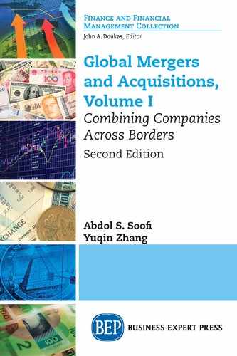
Now suppose the cash flows for the company in Example 7.1 are constant. Calculate the NPV of the company.

Accordingly, given the constant rate of growth in revenue and cost of capital, the NPV of the firm is negative.

Now let us assume k = 0.30. Calculate V₀:

What are the implications of the results of this example? First, a positive PV requires satisfaction of two conditions: m (1−T) < I and k < g. Second, a positive NPV will be guaranteed if m (1−T) >I and k > g.

Summary

This chapter dealt with the valuation of a company by discussing alternative methods of corporate valuation. Specifically, comparable companies, comparable transactions, and capital budgeting methods were considered. Moreover, in examining the capital budgeting approach, DCFs and NPV of valuation under different assumptions concerning revenue growth were reviewed.